A solution of (4.13) with  excitation ports, defined
between the cover and the bottom plane (Figure 4.2), relates the port
voltages
excitation ports, defined
between the cover and the bottom plane (Figure 4.2), relates the port
voltages
 on the ports with index
  to the currents
 on the ports with index
  by the impedance matrix
  . The
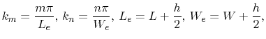
coordinates of port i and port j are
. The
coordinates of port i and port j are
 and
and
 respectively.
 with with |
(4.17) |
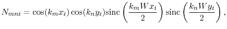
An analytical solution for rectangular parallel planes with four open edges depicted in
Figure 4.2 was presented by [42]. In this solution, the
coefficients of the impedance matrix in (4.17) are
![$\displaystyle Z_{ij}=\frac{j\omega\mu
h}{L_{e}W_{e}}\sum_{m=0}^{\infty}\sum_{n=0}^{\infty}\left[\frac{L_{mn}N_{mni}N_{mnj}}{{k_{m}^2+k_{n}^2-k^2}}
\right],$](img273.png) |
(4.18) |
with
 |
(4.19) |
 |
(4.20) |
 |
(4.21) |
 |
(4.22) |
and
 |
(4.23) |
Figure 4.2:
Rectangular, parallel metallic planes with four open edges.
Equation (4.18) contains the port impedance matrix
elements.
|
![\includegraphics[width=13cm,viewport=130 595 500 755,clip]{{pics/Open_Edges.eps}}](img279.png) |
In (4.18)
 denotes the wave number, with the
speed of light
denotes the wave number, with the
speed of light  .
.  and
and  are the effective plane length and width,
respectively. These effective dimensions consider the fringing fields at the cavity edges
according to [45].
[43] also provides an analytical solution for equilateral triangular parallel
planes with three open edges. Chapter 7 of this
work presents an analytical solution for rectangular parallel planes with one open and
three closed edges. This is a powerful solution for predesign investigations of the
radiated emissions from the slot of a slim cubical enclosure, because discussion of the
bias functions of the model provides direct information about the influence of the source
position on the emission level.
are the effective plane length and width,
respectively. These effective dimensions consider the fringing fields at the cavity edges
according to [45].
[43] also provides an analytical solution for equilateral triangular parallel
planes with three open edges. Chapter 7 of this
work presents an analytical solution for rectangular parallel planes with one open and
three closed edges. This is a powerful solution for predesign investigations of the
radiated emissions from the slot of a slim cubical enclosure, because discussion of the
bias functions of the model provides direct information about the influence of the source
position on the emission level.
The analytical method of [43] enables the calculation of parallel plane
cavities with fairly arbitrary shapes by connecting rectangular or equilateral triangular
parallel-plane segments. This method is illustrated in Figure 4.3.
Figure 4.3:
Three rectangular cavities are connected together with interface ports.
|
![\includegraphics[width=13cm,viewport=130 630 500
755,clip]{{pics/Port_Connection.eps}}](img282.png) |
C. Poschalko: The Simulation of Emission from Printed Circuit Boards under a Metallic Cover