2.4.2 Boltzmann Transport Equation

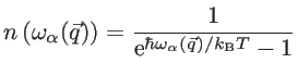
At equilibrium, the distribution of phonons in branch $\alpha$ and wavevector $\vec{q}$ is given by the Bose-Einstein distribution function $n(\omega)$ :

$$n\left( \omega_{\alpha}(\vec{q}) \right)=\frac{1}{\mathrm{e}^{\hbar \omega_{\alpha}(\vec{q})/k_{\mathrm{B}}T}-1}$$ (2.59)

Under non-equilibrium conditions, the distribution of phonons deviates from its equilibrium distribution, and transport of phonons is computed using the Boltzmann transport formalism. The non-equilibrium distribution function $\overline{n}(t,\vec{r},\omega)$ , in general, is a function of time $t$ and position $\vec{r}$ . The BTE can be written as:

$$\frac{\partial \overline{n}}{\partial t}+\vec{v} \cdot \nabla_{\v... ...rline{n}=\left( \frac{\partial \overline{n}}{\partial t}\right)_{\mathrm{scat}}$$ (2.60)

and for the steady state:

$$\vec{v} \cdot \nabla_{\vec{r}}\overline{n}=\left( \frac{\partial \overline{n}}{\partial t}\right)_{\mathrm{scat}}$$ (2.61)

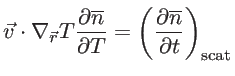
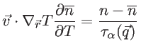
Under a temperature gradient, the BTE can be written as [60]:

$$\vec{v} \cdot \nabla_{\vec{r}}T \frac{\partial \overline{n}}{\partial T}=\left( \frac{\partial \overline{n}}{\partial t}\right)_{\mathrm{scat}}$$ (2.62)

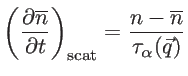
In the relaxation time approximation, the change of the distribution function due to the scattering events can be given by:

$$\left( \frac{\partial \overline{n}}{\partial t}\right)_{\mathrm{scat}}=\frac{n-\overline{n}}{\tau_{\alpha}(\vec{q})}$$ (2.63)

and therefore

$$\vec{v} \cdot \nabla_{\vec{r}}T \frac{\partial \overline{n}}{\partial T}=\frac{n-\overline{n}}{\tau_{\alpha}(\vec{q})}$$ (2.64)

where $\tau_{\alpha}(\vec{q})$ is the relaxation time of phonons of frequency $\omega_{\alpha}(\vec{q})$ . In this work we use a linearized form of Eq. 2.64, which assumes that the temperature gradient causes only a small deviation from Bose-Einstein distribution function [61,62], so that:

$$\frac{\partial \overline{n}}{\partial T}\approx \frac{\partial n}{\partial T}=\frac{\hbar \omega_{\alpha}(\vec{q})}{k_{\mathrm{B}}T^2}n(n+1)$$ (2.65)

and

$$\overline{n}=\frac{1}{\mathrm{e}^{\left( \hbar \omega_{\alpha}(\v... ...l (\hbar \omega)}\right)=n+\frac{\Psi_{\alpha}(\vec{q})n(n+1)}{k_{\mathrm{B}}T}$$ (2.66)

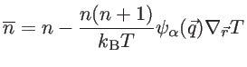
where $\Psi_{\alpha}(\vec{q})$ shows the deviation from the equilibrium distribution. Then, one may eliminate the temperature gradient using $\Psi_{\alpha}(\vec{q})=-\psi_{\alpha}(\vec{q})\nabla_{\vec{r}}T$ and write:

$$\overline{n}=n-\frac{n(n+1)}{k_{\mathrm{B}}T}\psi_{\alpha}(\vec{q})\nabla_{\vec{r}}T$$ (2.67)

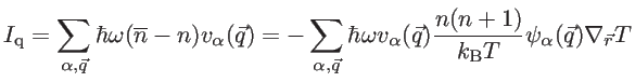
Since the equilibrium distribution does not carry any heat flux, the heat flux equals to [62]:

$$I_{\mathrm{q}}=\sum_{\alpha,\vec{q}}\hbar \omega (\overline{n}-n)... ...\vec{q}) \frac{n(n+1)}{k_{\mathrm{B}}T}\psi_{\alpha}(\vec{q})\nabla_{\vec{r}} T$$ (2.68)

On the other hand, it holds the differential form of Fourier's law:

$$I_{\mathrm{q}}=-\kappa_l \nabla T$$ (2.69)

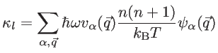
Therefore, one can obtain the lattice thermal conductivity as:

$$\kappa_l=\sum_{\alpha,\vec{q}}\hbar \omega v_{\alpha}(\vec{q}) \frac{n(n+1)}{k_{\mathrm{B}}T}\psi_{\alpha}(\vec{q})$$ (2.70)

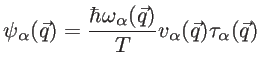
Under the single-mode relaxation time (SMRT) approximation [62], $\psi_{\alpha}(\vec{q})$ follows from the linearized BTE (Eqs. 2.64-2.66) as:

$$\psi_{\alpha}(\vec{q})=\frac{\hbar \omega_{\alpha}(\vec{q})}{T}v_{\alpha}(\vec{q}) \tau_{\alpha}(\vec{q})$$ (2.71)

Here, $\tau_{\alpha}(\vec{q})$ is the scattering time in SMRT approximation. Therefore, Eq. 2.70 becomes

$$\kappa_l=\sum_{\alpha,\vec{q}}\hbar \omega v_{\alpha}(\vec{q})^2 \tau_{\alpha}(\vec{q}) \frac{\partial n}{\partial T}$$ (2.72)