Alexander Grill Dipl.-Ing. Publications

In single defect measurements, the individual defects are commonly identified by clustering the observed step-heights into spectral maps. For time-dependent defect spectroscopy measurements, the spectral maps can easily be retrieved by plotting the step-heights versus the observed emission times. For random telegraph noise (RTN) signals, the time differences between adjacent capture and emission events of the same defect have to be calculated before constructing the spectral maps. The spectral maps are then binned into histograms based on their step-heights, and multivariate exponential distributions are used to extract the mean capture and emission times. One example for RTN observed in an GaN/AlGaN-fin high-electron-mobility transistors can be seen in Fig. 1.
Usually, the calculations of the time differences are done by using some sort of state machine, which calculates the delta times using the observed step-heights and their direction as parameters. If, for example, emissions from multiple traps have similar step-heights, or more complex Markov chains including thermal emissions with no charge transfer are observed, the design of the state machine becomes more and more unfeasible.
A Hidden Markov Model (HMM), capable of dealing with arbitrarily shaped Markov chains of multiple defects, helps to overcome this problem. Once the defects contributing to the RTN signal are specified, the HMM is trained with the measurement data and directly provides the step-heights and time constants of the individual defects in a maximum-likelihood manner. Other benefits are the ability to also simulate RTN signals and immunity to noisy measurement data.
The main drawbacks of HMM are that the Markov chain of the defect has to be chosen beforehand, and the training relies on absolute voltage levels, which makes it prone to long-term drift. The latter problem is mitigated by using a sophisticated baseline estimation algorithm during training.
Fig. 2 shows an example system consisting of a four-state defect, including one thermal state and a two-state defect, used for a model benchmark against various influences, together with a resulting trace. The robustness of the HMM extraction (100 seeds) against Gaussian measurement noise is proven by Fig. 3. The errors are negligible up to a normalized noise level of approximately 0.5, corresponding to a peak-to-peak noise of approximately the step-height of the dominant defect.
The robustness against long-term drift is shown in Fig. 4. The drift was constructed using random walks to rule out any systematic influence on the shape of the drift. It can be seen that the extraction works very well up to approximately a root mean square (RMS) value of 10 of the drift. Above that value, the baseline correction algorithm starts to break down, and the emissions are attributed to the wrong states of the Markov chain.

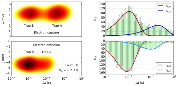
Fig. 1: Left: After step detection and the extraction of the delta times for capture and emission events, a spectral map consisting of the step-heights versus the delta times is plotted. In order to extract the time constants of different defects, those spectral maps are split into one or more histograms by the observed step-heights. Right: The histograms of the capture (top) and emission (bottom) times show the number of transition events at a certain gate voltage and temperature. The capture and emission times of each individual trap can be obtained most reliably by fitting multivariate exponential distributions to the data.

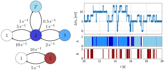
Fig. 2: Left: The Markov chains of a four-state defect with a hidden state and a two-state defect used for the model benchmarks. The charge state is neutral if the defect is in state 1, negative if in state 2’ or 2 and double negative in state 3. The step-heights are 5mV and 3mV. Right: Simulated emissions of the two defects combined. The RTN signal already looks quite complicated although only two defects are contributing. With conventional methods, the hidden state could not be determined.

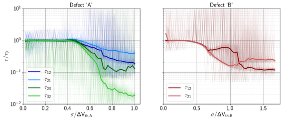
Fig. 3: The dependence of the normalized time constants on Gaussian noise. The results are close to their appropriate values up to a signal-to-noise ratio of about 0.5 to 0.6. This can be explained by the fact that around that value, the noise becomes larger than the step-height. For higher noise, the extracted time constants consistently decrease because large noise peaks become statistically relevant.

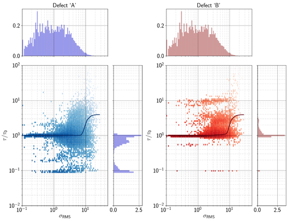
Fig. 4: The normalized time constants in relation to different baselines. The baselines were generated with random walks of different amplitudes. Up to an RMS value of about 8, the extracted times closely resemble the real values. The colormap used for the density plots is on a logarithmic scale to emphasize the spreading of the results at higher drift values.