3.8.3 Steady-State Kinetic Equations

Under steady-state condition the GREEN's functions depend on time differences. One usually FOURIER transforms the time difference coordinate, $\tau=t-t'$, to energy

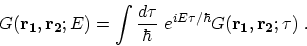$$\begin{array}{l}\displaystyle G({\bf {r}_1},{\bf {r}_2};E) =... ...iE\tau/\hbar} G({\bf {r}_1},{\bf {r}_2};\tau) \ . \end{array}$$ (3.70)

Under steady-state condition the quantum kinetic equations, (3.64), (3.65), and (3.69), can be written as [60]:

$$\begin{array}{l}\displaystyle \left[E-\hat{H}_0({\bf {r}_1})... ...2};E) \ = \ \delta_{{\bf {r}_1},{\bf {r}_2}} \ , \end{array}$$ (3.71)

$$\begin{array}{l}\displaystyle G^\mathrm{\lessgtr}({\bf {r}_1... ...;E) \ G^\mathrm{a}({\bf {r}_4},{\bf {r}_2};E) \ , \end{array}$$ (3.72)

where $\Sigma$ is the total self-energy. A similar transformation can be applied to self-energies. However, to obtain self-energies one has to first apply LANGRETH's rules and then FOURIER transform the time difference coordinate to energy. We consider the self-energies discussed in Section 3.6. The evaluation of the HARTREE self-energy due to electron-electron interaction is straightforward, since it only includes the electron GREEN's function. However, the lowest-order self-energy due to electron-phonon interaction contains the products of the electron and phonon GREEN's functions. Using LANGRETH's rules (Table 3.1) and then FOURIER transforming the self-energies due to electron-phonon interaction, (3.50) takes the form

$$\begin{array}{ll}\displaystyle \Sigma_\mathrm{el-ph}^{\gtrle... ...mbda} ({\bf q},\hbar\omega_{{\bf q},\lambda}) \ , \end{array}$$ (3.73)

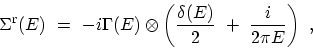
To calculate the retarded self-energy, however, it is more straightforward to FOURIER transform the relation $\Sigma^\mathrm{r}(\tau)=\theta(\tau)[\Sigma^\mathrm{>} (\tau)-\Sigma^\mathrm{<}(\tau)]$, see (3.52). By defining the broadening function $\Gamma$

$$\begin{array}{l}\displaystyle \Gamma({\bf r_1},{\bf r_2};E)=... ...{m} \Sigma^\mathrm{<}({\bf r_1},{\bf r_2};E) \ , \ \end{array}$$ (3.74)

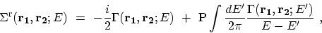
the retarded self-energy is given by the convolution of $-i\Gamma(E)$ and the FOURIER transform of the step function [33]

$$\begin{array}{l}\displaystyle \Sigma^\mathrm{r}(E) \ = \ -i\... ...c{\delta(E)}{2} \ + \ \frac{i}{2\pi E}\right) \ , \end{array}$$ (3.75)

where $\otimes$ denotes the convolution. Therefore, the retarded self-energy is given by [116]

$$\begin{array}{l}\displaystyle \Sigma^\mathrm{r}({\bf r_1},{\... ...}\frac{\Gamma({\bf r_1},{\bf r_2};E')}{E-E'} \ , \end{array}$$ (3.76)

where $\mathrm{P}$ stands for principal part.

M. Pourfath: Numerical Study of Quantum Transport in Carbon Nanotube-Based Transistors