


Next: 4. Doping of Group-IV-Based
Up: Dissertation Robert Wittmann
Previous: 2. Semiconductor Doping Technology
Subsections
3. Simulation of Ion Implantation
There are two methods, the analytical and the Monte Carlo method, which are
commonly used in modern TCAD tools for the simulation of ion implantation
processes. Mainly increasing accuracy requirements due to the continued
downscaling of device dimensions necessitate the transition from the simple
analytical simulation of ion implantation to the particle-based Monte Carlo
simulation for more and more applications. This chapter outlines fundamental
modeling concepts required for the physically based simulation of doping profiles.
The basic idea of the analytical approach is that the doping profile can be
approximated by a statistical distribution
function [45,46,42,47].
This function depends on a set of parameters which can be expressed by
characteristic parameters of the implanted dopant distribution, for instance,
the mean projected range  . The characteristic parameters, the so-called
moments, can be extracted from Monte Carlo calculation results or from
measured doping profiles. One-dimensional distribution functions can be
combined to multi-dimensional profiles by a convolution method which takes
a dose matching rule and numerical scaling into account. The analytical
simulation of profiles requires relatively little CPU-time, even in two and
three dimensions.
. The characteristic parameters, the so-called
moments, can be extracted from Monte Carlo calculation results or from
measured doping profiles. One-dimensional distribution functions can be
combined to multi-dimensional profiles by a convolution method which takes
a dose matching rule and numerical scaling into account. The analytical
simulation of profiles requires relatively little CPU-time, even in two and
three dimensions.
Due to the simplicity of the underlying concept, analytical implantation
tools cannot accurately predict doping profiles for complex targets, for
instance, multilayer targets or advanced devices with junction depths in
the range of a few nanometers. In a compound target like SiGe, range
predictions will be still worse, because the doping profiles additionally
depend on the germanium fraction of the alloy. In contrast to that, the
physics-based Monte Carlo method uses an atomistic approach and, therefore,
is able to simulate the channeling effect and the accumulation of point
defects during the implantation process in crystalline targets, as well as, e.g.,
shadowing effects arising from mask edges [15,17,42].
The Monte Carlo method imitates the implantation process by computing a large
number of individual ion trajectories in the target. The three-dimensional device
structures can be complex, with the only limitation being the computer memory
size which must hold all the interaction details of the target. The underlying
physical models are applicable for a wide range of implantation conditions
without the need for an additional calibration.
One drawback of the Monte Carlo method are long computing times, which is the
main reason why the use of Monte Carlo implantation tools is usually
avoided in technology optimization. However, the capability of accurately
predicting doping profiles can significantly reduce the development time for
a new CMOS technology. In particular next generation technology nodes in the
deep sub-100nm regime will put high demands on the accuracy of TCAD tools.
3.1 Physical Models
This chapter outlines the fundamental physics associated with the penetration
of energetic ions into solids. The moving ions lose energy to the solid, create
point defects, and after stopping they produce the final distribution in the
target. The Monte Carlo modeling of ion implantation allows the incorporation
of arbitarily complex physical models at an atomic level.
An ion which penetrates into a target loses energy constantly to the sea of
electrons. It may go many atomic layers, before there is a collision with a
target atom which is hard enough to displace that atom and create an interstitial
and vacancy pair. The energy required to push a target atom just far enough from
its lattice site so that it cannot pop back into its empty site is the
displacement energy  , which is approximately 15eV in silicon.
Fig. 3.1 shows different scenarios which can arise for ions shot into a
crystalline target material.
, which is approximately 15eV in silicon.
Fig. 3.1 shows different scenarios which can arise for ions shot into a
crystalline target material.
Assume an incident ion with atomic number  and energy
  has a collision
with a target atom of atomic number
has a collision
with a target atom of atomic number  . After the collision the incident atom
has energy
. After the collision the incident atom
has energy  and the struck atom has energy
  . A displacement
occurs if
. A displacement
occurs if  , so that the atom has enough energy to leave the
site. A vacancy occurs if both
, so that the atom has enough energy to leave the
site. A vacancy occurs if both  and . Both atoms
then become moving atoms of the cascade. If
and . Both atoms
then become moving atoms of the cascade. If  , then the atom
does not have enough energy and it will vibrate back to its site releasing
as phonons. If
, then the atom
does not have enough energy and it will vibrate back to its site releasing
as phonons. If  , , and
  , then the
incoming atom remain at the site and the collision is called a replacement
collision with released as phonons. This type of collision is common in
single element targets with large recoil cascades. If , ,
and
, then the
incoming atom remain at the site and the collision is called a replacement
collision with released as phonons. This type of collision is common in
single element targets with large recoil cascades. If , ,
and
 , then becomes an interstitial atom.
Figure 3.1:
The incident ions 'make way' for themselves by knocking
the target atoms out of their lattice sites, whereas recoil cascades are generated.
![\resizebox{0.64\linewidth}{!}{\rotatebox{0}{\includegraphics[clip]{figures/damage}}}](img235.png) |
Figure 3.2:
Principle of the Monte Carlo simulation method.
|
|
Ziegler et al. have demonstrated in [16] that the Monte Carlo
calculation of ion trajectories is a very feasible way for accurately simulating
the final ion distribution in crystalline silicon. Typically, Monte Carlo
programs calculate a large number of individual particle trajectories in a target.
Each particle history begins with a random starting position within the implantation
window, a given direction, and an ion beam energy  . Fig. 3.2 depicts
that a particle changes its direction as a result of nuclear collision events
and moves in straight free-flight-paths between collisions. The kinetic energy of
the particle is reduced as a result of nuclear and electronic energy losses, and
the history is terminated either when the energy drops below a specified value
. Fig. 3.2 depicts
that a particle changes its direction as a result of nuclear collision events
and moves in straight free-flight-paths between collisions. The kinetic energy of
the particle is reduced as a result of nuclear and electronic energy losses, and
the history is terminated either when the energy drops below a specified value
 or when the particle leaves the simulation domain.
The rate at which an ion loses energy depends on the target atom density
or when the particle leaves the simulation domain.
The rate at which an ion loses energy depends on the target atom density  (in
cm
(in
cm ) and on the nuclear and electronic stopping powers
  and
and  (in eVcm
 ),
),
![$\displaystyle \frac{\mathrm{d}E}{\mathrm{d}x}\; =\; - N_T\; \left[ S_n(E) + S_e(E) \right] \;.$](img240.png) |
(3.1) |
The nuclear and electronic stopping powers are assumed to be independent and
both are in general functions of energy.
3.1.2 Binary Collision Approximation
The interaction of the moving ion with an atomic nucleus of the target (nuclear
stopping) can be treated as an elastic collision process, whereas the
interaction with the electrons can be treated as an inelastic process without
any scattering effects (electronic stopping). The binary collision approximation
(BCA) assumes that only two charged particles, the moving ion (atomic number
, mass  , kinetic energy ) and one target atom (atomic number
, mass
, kinetic energy ) and one target atom (atomic number
, mass  ) are involved in one scattering process. While the moving
particle passes and is deflected, the stationary particle recoils
or at least activates thermal lattice vibrations. The distance between the
incident direction and the stationary particle is the impact parameter
) are involved in one scattering process. While the moving
particle passes and is deflected, the stationary particle recoils
or at least activates thermal lattice vibrations. The distance between the
incident direction and the stationary particle is the impact parameter  .
Fig. 3.3 shows the scattering variables in a two-body collision.
The unknown velocities
.
Fig. 3.3 shows the scattering variables in a two-body collision.
The unknown velocities  ,
,  and directions
  ,
,  from
the incident direction after the collision event can be found from the
conservation of energy (3.2) and momentum (3.3),
(3.4) in the laboratory system.
from
the incident direction after the collision event can be found from the
conservation of energy (3.2) and momentum (3.3),
(3.4) in the laboratory system.
Figure 3.3:
Classical two particle scattering process in the
laboratory system and in the center-of-mass system.
![\resizebox{1.1\linewidth}{!}{\rotatebox{0}{\includegraphics[clip]{figures/binscatter}}}](img247.png) |
For solving this two-body problem it is convenient to transform the scattering
process from the laboratory coordinates to the center-of-mass coordinate (CM)
system of ion and target atom. In Fig. 3.3, the CM system moves with
constant velocity  to the right. Equation (3.5) defines in such
a way that the total momentum of the CM system becomes zero. The basic reason
for this transformation is that the CM system reduces any two-body problem to
a one-body problem, because the total momentum of the particles is always zero
and the paths of the two particles are symmetric as shown in Fig. 3.3.
The single particle has the initial kinetic energy
to the right. Equation (3.5) defines in such
a way that the total momentum of the CM system becomes zero. The basic reason
for this transformation is that the CM system reduces any two-body problem to
a one-body problem, because the total momentum of the particles is always zero
and the paths of the two particles are symmetric as shown in Fig. 3.3.
The single particle has the initial kinetic energy  (3.6) and moves
with a reduced mass
(3.6) and moves
with a reduced mass  (3.7) and velocity in a stationary potential
V(r) which is centered at the origin of the CM coordinates.
(3.7) and velocity in a stationary potential
V(r) which is centered at the origin of the CM coordinates.
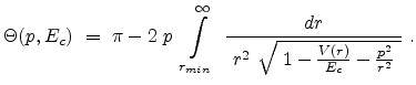
Ziegler derivates the particle scattering path by using Lagrangian mechanics in
polar coordinates in [17]. The result is the famous ``scattering
integral'' (3.8) which allows to evaluate the scattering angle  in the CM system. The angle depends on the energy , the interatomic
potential
in the CM system. The angle depends on the energy , the interatomic
potential  , and the impact parameter . The distance of minimum approach
between the two particles is denoted as
, and the impact parameter . The distance of minimum approach
between the two particles is denoted as  (see Fig. 3.3), which is
determined by the real root of the denominator in (3.8).
(see Fig. 3.3), which is
determined by the real root of the denominator in (3.8).
 |
(3.8) |
The inverse transformation leads to the scattering angle of the ion
(3.9), the angle of the recoil (3.10), and the loss in
energy of the ion,  , which is equal to the recoil energy (3.11).
The scattering integral (3.8) cannot be calculated analytically for
interatomic screening potentials and a numerical integration would be too
time-consuming, since a simulated ion undergoes typically 100 to 1000 collisions.
Solutions to this problem are to use an analytical approximation formula or a
lookup table method. The used method is of critical importance in terms of
accuracy and efficiency for the Monte Carlo calculation.
The only non-trivial quantity in equation (3.8) is the interaction
potential between the ion and the target atom. The potential
is a repulsive Coulomb potential between the two positively charged nuclei,
which is screened by surrounding electrons. The effect of the electrons is
described by a dimensionless screening function  which is less than
one.
which is less than
one.
 |
(3.12) |
and are the atomic numbers of the involved particles,  is
the elementary charge, and
is
the elementary charge, and
 is the dielectric constant.
Well-known older screening functions are the Bohr potential [48],
the Thomas-Fermi potential [49], the Moliere [50],
and the Lenz-Jensen approximation [51]. Ziegler, Biersack, and Littmark
performed the calculation of the interatomic potentials for 522 atom pairs.
Based on these calculations they could derive the universal screening
potential which is suitable for arbitrary atom pairs [17].
is the dielectric constant.
Well-known older screening functions are the Bohr potential [48],
the Thomas-Fermi potential [49], the Moliere [50],
and the Lenz-Jensen approximation [51]. Ziegler, Biersack, and Littmark
performed the calculation of the interatomic potentials for 522 atom pairs.
Based on these calculations they could derive the universal screening
potential which is suitable for arbitrary atom pairs [17].
The equation (3.13) for the universal screening function  consists
of four fitted exponential terms and uses the scaled radius
consists
of four fitted exponential terms and uses the scaled radius  as its argument.
Ziegler, Biersack, and Littmark introduced the scaled radius according to
(3.14), where
as its argument.
Ziegler, Biersack, and Littmark introduced the scaled radius according to
(3.14), where  is the real radius,
  is the universal screening
length, and
is the universal screening
length, and
 is the Bohr radius. In the
literature the universal potential is known as Ziegler-Biersack-Littmark (ZBL)
potential.
is the Bohr radius. In the
literature the universal potential is known as Ziegler-Biersack-Littmark (ZBL)
potential.
Figure 3.4:
Universal screening potential and other approximations.
![\resizebox{0.8\linewidth}{!}{\rotatebox{0}{\includegraphics[clip]{figures/unipot}}}](img283.png) |
Table 3.1:
Debye temperature  and corresponding average vibration
amplitude
and corresponding average vibration
amplitude  .
.
| Method |
(K) |
 at 300K at 300K |
| Specific heat |
645 |
0.065 |
| Channeling experiment |
490 |
0.083 |
| Simulation of ion implantation |
450 |
0.090 |
|
Thermal vibrations displace the lattice atoms from their ideal lattice positions
and they have been identified as source of the dechanneling mechanism, unless
the crystalline target contains considerable damage [52,53].
The approximation of a spherically symmetric Gaussian distribution
 can be used to describe the displacement of
atoms from their rest position.
can be used to describe the displacement of
atoms from their rest position.
![$\displaystyle f(\Delta x, \Delta y, \Delta z) = \frac{1}{\sqrt[3]{2\pi\sigma^2}...
...m{exp} \left(-\frac{\Delta x^2 + \Delta y^2 + \Delta z^2}{2\sigma^2}\right) .$](img286.png) |
(3.15) |
The standard deviation of the atomic displacement
 from the rest position can be adjusted
according to the Debye theory [54], which is in good agreement
with X-ray diffraction experiments [55]. This theory uses an empirical
parameter, the Debye temperature , which can be determined with the aid of
specific heat measurements [56], by channeling experiments [57],
or by comparison of simulated profiles with SIMS data [58], as summarized
in Table 3.1 for silicon at a wafer temperature of 300K.
from the rest position can be adjusted
according to the Debye theory [54], which is in good agreement
with X-ray diffraction experiments [55]. This theory uses an empirical
parameter, the Debye temperature , which can be determined with the aid of
specific heat measurements [56], by channeling experiments [57],
or by comparison of simulated profiles with SIMS data [58], as summarized
in Table 3.1 for silicon at a wafer temperature of 300K.
Fig. 3.5 shows a sample size of 10000 atom vibration amplitudes which are used
for the Monte Carlo calculation of ion trajectories in MCIMPL-II. The simulator
uses an average vibration amplitude
 according
to a Debye temperature of 490K to model the motion of the atoms in silicon.
Note that the random variates from the Gaussian distribution presented in
Fig. 3.5 are derived from a random-number generator which produces uniformly
distributed random variates in the interval
according
to a Debye temperature of 490K to model the motion of the atoms in silicon.
Note that the random variates from the Gaussian distribution presented in
Fig. 3.5 are derived from a random-number generator which produces uniformly
distributed random variates in the interval ![$ [0, 1]$](img289.png) . The fast polar method
is used to generate originally random variates in pairs from the normal distribution
contained in the interval
. The fast polar method
is used to generate originally random variates in pairs from the normal distribution
contained in the interval
![$ [-\infty, \infty]$](img290.png) with mean
with mean  and standard
deviation
and standard
deviation
 , as described in [59].
Figure 3.5:
Gaussian distribution of the atom vibration amplitudes in
MCIMPL-II.
![\resizebox{0.8\linewidth}{!}{\rotatebox{0}{\includegraphics[clip]{figures/atomvib}}}](img293.png) |
3.1.3 Electronic Stopping Power
The electronic stopping power of the target is complicated and not fully understood
up to now, since several physical processes contribute to the electronic energy
loss [16]:
- Direct kinetic energy transfer to target electrons, mainly due to
electron-electron collisions.
- Excitation of band- or conduction-electrons (effect on weakly bound or
non-localized target electrons).
- Excitation or ionization of target atoms (effect on localized electrons).
- Excitation, ionization, or electron-capture of the projectile.
The electronic stopping models used for Monte Carlo implantations into silicon
can be classified as non-local or local. While non-local models assume that the
electronic energy loss is independent of the relative positions of the ion and
the target atoms [60,16], local models take such a dependence
into account, using either the impact parameter of the collisions [61]
or the local electron concentration along the ion path [62].
Hobler et al. proposed an empirical electronic stopping model for the implantation
into crystalline silicon [63], which is based on the Lindhard electronic
stopping model and an impact parameter approach.
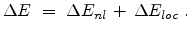
In the Hobler model the total electronic energy loss is composed of a
non-local part which dominates in the case of large impact parameters (channeling
ions) and a local part which is considered at every collision.
 |
(3.16) |
The non-local part
 is proportional to the the path length
  traveled by the ion between two nuclear collision events in a target material with
atomic density
traveled by the ion between two nuclear collision events in a target material with
atomic density  .
.
![$\displaystyle \Delta E_{nl} = N \; S_e \; \Delta R \cdot\left[ x_{nl} + x_{loc}...
...\frac{p_{max}}{a}\right) \mathrm{exp}\left(-\frac{p_{max}}{a}\right)\right] .$](img298.png) |
(3.17) |
The local part
 is exponentially proportional to the impact parameter as proposed
by Oen and Robinson in [61].
is exponentially proportional to the impact parameter as proposed
by Oen and Robinson in [61].
 |
(3.18) |
The term in equation (3.17) containing  approximates the local
electronic energy loss due to collisions with impact parameters larger than
approximates the local
electronic energy loss due to collisions with impact parameters larger than  .
The electronic stopping power
.
The electronic stopping power  is assumed to be velocity proportional
in (3.19). Lindhard et al. proposed the expression (3.20) for the
coefficient
is assumed to be velocity proportional
in (3.19). Lindhard et al. proposed the expression (3.20) for the
coefficient  [60], which considers the properties of the ion
species and the target material.
[60], which considers the properties of the ion
species and the target material.
and are the charge and the mass of the implanted particle, is
the atomic charge in single-element targets,  is the Bohr radius, and
the kinetic energy of the particle. The Lindhard correction factor
is the Bohr radius, and
the kinetic energy of the particle. The Lindhard correction factor  is used to empirically adjust the strength of the electronic stopping.
The screening length
is used to empirically adjust the strength of the electronic stopping.
The screening length  is expressed by the value
 in [61], where is the screening length used for the interatomic
screening potential in (3.14). Hobler et al. multiplied the length by a
screening pre-factor
in [61], where is the screening length used for the interatomic
screening potential in (3.14). Hobler et al. multiplied the length by a
screening pre-factor  according to
 |
(3.21) |
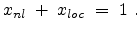
The parameters  and are the non-local and the local fraction
of the total electronic stopping power which requires the relation (3.22)
to hold.
and are the non-local and the local fraction
of the total electronic stopping power which requires the relation (3.22)
to hold.
 |
(3.22) |
The non-local fraction depends on the energy and can be modeled by
a power law,
 |
(3.23) |
Table 3.2:
Energy limits for the velocity proportional
electronic stopping power [42].
| Dopant species |
Energy limit (MeV) |
| Arsenic |
194.1 |
| Boron |
2.2 |
| Phosphorus |
28.0 |
|
where the empirical parameters  and are the non-local pre-factor
and non-local power.
Lindhard indicated that the electronic stopping power is only proportional
to the ion velocity up to a maximal energy which is shown for some important ion
species in Table 3.2.
and are the non-local pre-factor
and non-local power.
Lindhard indicated that the electronic stopping power is only proportional
to the ion velocity up to a maximal energy which is shown for some important ion
species in Table 3.2.
The drawback of the empirical Hobler model is that many parameters have to be
fitted, in particular for crystalline materials. Hobler has demonstrated for
boron implantations in crystalline silicon [64] that the accuracy
of the empirical model is better than that of the purely electron-density-based
model. The Hobler model requires less additional computational effort since the
impact parameter which is used by the BCA algorithm to determine the nuclear
energy loss can be applied to calculate the electronic energy loss. Both the
nuclear and the electronic stopping powers depend on the energy and contribute
to the total stopping. Fig. 3.6 demonstrates the slowing down of boron
ions with an initial energy of 40keV. Note that the nuclear stopping has its
maximum at 3keV and the electronic stopping dominates for higher energies.
Figure 3.6:
Average nuclear and electronic stopping powers
and for a 40keV boron implantation into silicon, analyzed with
MCIMPL-II.
![\resizebox{0.77\linewidth}{!}{\rotatebox{0}{\includegraphics[clip]{figures/energyloss}}}](img317.png) |
Summarizing, it can be said that the electronic stopping is dominant for higher
energies, lighter ions, and under channeling conditions.
3.1.4 Damage Generation
The nuclear stopping process of energetic ions in crystalline targets displaces
atoms from their lattice sites. If the ion implantation dose is high enough, a
continuous amorphous layer can be formed in a silicon wafer beneath the surface.
A so-called Frenkel pair or Frenkel defect is formed when a
displaced target atom forms an interstitial and leaves a vacancy behind at its
original lattice site [29]. The point defects in the target accumulate
during the implantation process and influence the trajectories of subsequently
implanted ions. In addition, the generated point defects cause a transient
enhanced diffusion (TED) effect of dopant atoms during the RTA annealing process.
Due to the fact that it is difficult to measure damage concentrations in crystals,
the simulation of implantation induced point defects as well as the identification
of amorphized regions in the device are very beneficial for modern CMOS process
engineering.
The generation of point defects can be modeled by the analytical modified
Kinchin-Pease model or by the computationally intensive Follow-Each-Recoil
method.
Modified Kinchin-Pease Model
The modified Kinchin-Pease model assumes that the number of displaced atoms
(Frenkel pairs) in a collision cascade is a function of the transferred
energy from the ion to the primary recoil atom [65,66].
In this theory, the defect producing energy  is obtained from the kinetic
energy of the primary knock-on recoil, reduced for the electronic loss by all
recoils comprising the cascade. The recoils themselves are not individually
followed in this computationally fast approach. It was found in [63]
that experimental results can be well described by the modified Kinchin-Pease
model together with a model for point defect recombination. The defect
recombination which takes place in a recoil cascade can be modeled empirically
by using the local point defect concentration.
is obtained from the kinetic
energy of the primary knock-on recoil, reduced for the electronic loss by all
recoils comprising the cascade. The recoils themselves are not individually
followed in this computationally fast approach. It was found in [63]
that experimental results can be well described by the modified Kinchin-Pease
model together with a model for point defect recombination. The defect
recombination which takes place in a recoil cascade can be modeled empirically
by using the local point defect concentration.
The electronic energy loss is calculated according to Lindhard's
theory [67] using the analytical approximation of
Robinson [68] to the universal function
 .
The ``damage energy'' is calculated from the initial energy
of the primary recoil by
.
The ``damage energy'' is calculated from the initial energy
of the primary recoil by
where  and
and  are the atomic number and mass of the recoil atoms, and the reduced
energy
are the atomic number and mass of the recoil atoms, and the reduced
energy
 is a dimensionless quantity. The number of generated
Frenkel pairs
is a dimensionless quantity. The number of generated
Frenkel pairs  in a recoil cascade can be calculated from the energy
using a constant displacement efficiency
in a recoil cascade can be calculated from the energy
using a constant displacement efficiency
 in the modified
Kinchin-Pease damage generation formula, given by
in the modified
Kinchin-Pease damage generation formula, given by
Figure 3.7:
Number of Frenkel pairs generated by a primary knock-on atom
in silicon assuming  eV, plotted for two different energy ranges.
|
|
The primary recoil atom produces only lattice vibrations if the damage energy
is below the displacement energy . The curves in
Fig. 3.7 show the number of produced point defects for
damage cascades in silicon as a function of the transferred energy
without considering pre-existing point defects, as calculated by the modified
Kinchin-Pease model.
The recombination between interstitials and vacancies has to be taken into
account in order to realistically calculate the produced amount of point
defects [63]. The recombination within a collision cascade can be
described by a constant fraction  of Frenkel pairs surviving the
spontaneous self-annealing process due to beam-induced heating of the wafer.
If is the number of point defects generated in a recoil cascade,
then the average number of point defects surviving recombination within the
cascade is given by
of Frenkel pairs surviving the
spontaneous self-annealing process due to beam-induced heating of the wafer.
If is the number of point defects generated in a recoil cascade,
then the average number of point defects surviving recombination within the
cascade is given by
 . The correction parameter
depends on the ion species since heavy ions produce damage more
efficiently by overlapping of large cascades than lighter ions. A light ion
produces typically small cascades due to small transfer energies, where
recombination becomes more likely. The recombination with point defects of
previously generated damage cascades can be included by an additional factor
. The correction parameter
depends on the ion species since heavy ions produce damage more
efficiently by overlapping of large cascades than lighter ions. A light ion
produces typically small cascades due to small transfer energies, where
recombination becomes more likely. The recombination with point defects of
previously generated damage cascades can be included by an additional factor
 which depends on the recombination probability
  defined
in (3.33). The average number of stable point defects
defined
in (3.33). The average number of stable point defects  is linked to the number of generated point defects according to
The factor is obtained by considering the four possible cases for a
Frenkel pair having survived recombination within the recoil cascade. In the
first case, the generated Frenkel pair (both components) recombines with a
pre-existing Frenkel pair, which reduces the total number of Frenkel pairs
by one. The probability for this process is  . In the second case,
which occurs with the probability
. In the second case,
which occurs with the probability
 , the generated
Frenkel pair survives, resulting in an addditional Frenkel pair. In the
third and forth case either the interstitial or the vacancy survives while the
other one recombines, resulting in no change of the total Frenkel pair number.
Adding this changes with their probabilities yields
, the generated
Frenkel pair survives, resulting in an addditional Frenkel pair. In the
third and forth case either the interstitial or the vacancy survives while the
other one recombines, resulting in no change of the total Frenkel pair number.
Adding this changes with their probabilities yields
 as the
net average fraction of point defects surviving recombination with previously
generated point defects.
The recombination probability is proportional to the concentration
of already existing vacancies and interstitials and it has a species dependent
saturation level
as the
net average fraction of point defects surviving recombination with previously
generated point defects.
The recombination probability is proportional to the concentration
of already existing vacancies and interstitials and it has a species dependent
saturation level  as given in (3.33). Assuming equal local
concentrations of vacancies and interstitials,
as given in (3.33). Assuming equal local
concentrations of vacancies and interstitials,  , the probability
has to be equal to the probability of survival
, the probability
has to be equal to the probability of survival
 at
the saturation concentration, leading to
at
the saturation concentration, leading to
 for
for
 .
Substituting (3.32) and (3.33) into (3.31) and
assuming , the number of stable point defects are finally
obtained by
.
Substituting (3.32) and (3.33) into (3.31) and
assuming , the number of stable point defects are finally
obtained by
 |
(3.34) |
In principle, the displaced atoms can be placed on tetrahedral interstitial sites
(tetrahedral interstitial model) [69], on random positions (random
model) [70], or on random positions within spheres around the
tetrahedral interstitial sites. In [63], Hobler et al. placed the
silicon interstitials on random positions within the maximum impact parameter
from the ion path in the plane perpendicular to the ion's direction
of motion. From the comparison of simulations and experiments they found that the
silicon interstitials are rather randomly distributed in the crystal lattice
than located at tetrahedral interstitial sites.
The modified Kinchin-Pease model can only estimate the number of vacancies
produced in a collision cascade and, therefore, this damage model assumes the
same local concentration for the interstitials. There is a small offset between
the local vacancy and interstitial concentrations, since a vacancy stays
at the position where the recoil has been generated whereas an interstitial
typically comes to rest somewhere slightly deeper in the target.
This results in an interstitial profile with its peak at a slightly deeper
position than the peak of the corresponding vacancies.
The Follow-Each-Recoil method calculates the trajectories of all recoiling
atoms in a collision cascade. In the full cascade simulation, the nuclear
and electronic loss of a recoil is calculated in the same way as for an
implanted ion just with different physical properties. This approach requires
a tremendous computational effort, since a cascade can be in the range of
thousand displaced atoms in silicon, as demonstrated for high energies of
the primary recoil in the right plot of Fig. 3.7.
The advantage of the Follow-Each-Recoil method is that the location of the
interstitials can be accurately calculated as well as pollution effects can
be estimated. A pollution occurs in a semiconductor device, for instance,
if implanted ions push oxygen atoms from an isolation layer into the active
area of the device [71].
For a rigorous study of doping profiles for advanced semiconductor devices it
is mandatory to consider crystalline materials and arbitrary three-dimensional
geometries. The Monte Carlo ion implantation simulator MCIMPL-II was used
for the simulation of doping profiles throughout this thesis. Therefore, a brief
description of the simulator is presented in this section. The simulator has
been developed on the basis of MCIMPL [15] at the Institute for
Microelectronics. In contrast to its predecessor, MCIMPL-II has a flexible
object-oriented architecture and uses the functionality of the Wafer-State-Server
library [72]. MCIMPL-II can be easier extended to new materials,
while MCIMPL was originally just designed for the implantation into silicon.
Hobler started the project in 1986 by implementing the fundamental physical
models and by calibrating the models for the most important dopant species used
in silicon technology [73]. Stippel extended the simulator to three
dimensions [74] and Bohmayr implemented the Trajectory-Split
method [75]. Hössinger included the Follow-Each-Recoil method
in MCIMPL [42]. When he designed MCIMPL-II, he replaced
the simple data management of MCIMPL by a better handling of the simulation
data for a fast point location in heavily non-planar device
structures [76]. In the scope of this work, the postprocessing
of raw Monte Carlo data in MCIMPL-II was improved, and a grid-generator was
implemented to allow a fast simulation of one-dimensional doping profiles
which is particularly necessary for calibration purposes.
The current status is that MCIMPL-II can be used for one- and three-dimensional
implantation applications. Two-dimensional applications can be modeled by using
two-and-a-half dimensional device geometries with a small depth dimension.
The simulator can handle arbitrarily shaped device structures including overhang
structures. The simulated structure can be composed of several amorphous and
crystalline material segments. Various amorphous materials can be simulated,
for instance, SiO , Si
, Si N
N , TiN, or TaN, which are typically used in
CMOS processing. Several crystalline material segments can also be used in one
simulation domain with the restriction that the crystal orientation has to be
identical in all segments. In this work the simulator has been extended from
crystalline silicon to Si
, TiN, or TaN, which are typically used in
CMOS processing. Several crystalline material segments can also be used in one
simulation domain with the restriction that the crystal orientation has to be
identical in all segments. In this work the simulator has been extended from
crystalline silicon to Si
 Ge
Ge
 alloys of arbitrary
germanium content in the range from silicon to germanium. Polycrystalline
materials are treated as amorphous materials in which the crystalline structure
of the grains is neglected. This is not really a restriction, since
low-resistivity polysilicon for gates or interconnects is usually processed by
deposition of amorphous silicon, followed by high-dose ion implantation doping,
and finishing annealing.
alloys of arbitrary
germanium content in the range from silicon to germanium. Polycrystalline
materials are treated as amorphous materials in which the crystalline structure
of the grains is neglected. This is not really a restriction, since
low-resistivity polysilicon for gates or interconnects is usually processed by
deposition of amorphous silicon, followed by high-dose ion implantation doping,
and finishing annealing.
The Monte Carlo calculation of ion trajectories in crystalline targets uses
substantially only two random processes. The first one is applied to achieve
equally distributed starting points of ion trajectories within the implantation
window and the second one is used to imitate the thermal vibrations of the
target atoms. While the simulated ion moves through the target the simulator
uses locally either a crystalline or an amorphous model for searching the next
collision partner of the ion. The application of the amorphous model in crystalline
targets is performed with a certain probability which depends on the amount of
already generated damage in the crystal. Thus the transition from the crystalline
to the amorphous state of a region is taken into account, which is caused by the
accumulation of point defects during the implantation process. Note that the
Monte Carlo simulation of ion implantation without consideration of damage is
a static problem where the passage of time plays no role. In consideration of
damage accumulation over time the Monte Carlo simulation becomes dynamic.
In order to improve the performance, the simulator uses histogram cells aligned
on an orthogonal grid to count the number of implanted ions and of generated
point defects. The doping or damage concentration within a cell is obtained by
the number of particles contained in the cell divided by the volume of the cell.
However, the ion implantation process is accurately simulated by computing a
large number of individual ion trajectories in the target. Being based on
appropriately scaled random numbers, the results obtained with the Monte Carlo
method are never exact, but they converge to the characteristics of the
underlying physical models by increasing the number of simulated ions.
The statistical error of Monte Carlo results vanishes for a sample size
 .
.
Figure 3.8:
Schematic diagram of the Monte Carlo simulation with MCIMPL-II.
![\resizebox{0.98\linewidth}{!}{\rotatebox{0}{\includegraphics[clip]{figures/dataflow}}}](img362.png) |
The principle of simulator operation can be grouped into the following three
sections:
- Initialization of the internal data structures
- Physical Monte Carlo simulation of ion trajectories
- Transfer of the doping data to an unstructured grid
The input device structure for implantation is provided as a file in the WSS
(Wafer State Server) format [77], which contains all geometry and
material information of the simulation domain. Thereby the dimension of the
simulation is specified by the input WSS file. Additionally, the input file can
contain implantation data from previous implantation steps. The implantation
conditions and simulation parameters, for instance, the desired number of
simulated ions are specified by user defined command-line parameters.
A description of the simulator command-line interface is provided in [42].
Fig. 3.8 shows schematically the simplified simulation data flow from
the input file to the output file.
The simulation is started by initializing the histogram for the Monte Carlo
simulation. When histogram cells are set up, they are initialized with data from
previous implantation steps and they are continuously updated when damage is
generated by an ion. Thereby damage accumulation from several ion implantation
steps is automatically considered as well as damage accumulation within a single
implantation step. The incoming dopant ions are slowed down due to the nuclear
and electronic stopping power of the target material. The final position of an
implanted ion is reached where it has lost its kinetic energy.
After performing the Monte Carlo calculation of all ion trajectories, the dopants,
vacancies and interstitials are stored in histograms. A sophisticated
smoothing algorithm based on the Bernstein polynomial
approximation [78] is applied in order to reduce the statistical
fluctuation of raw Monte Carlo results.
The smoothed data are then translated from the internal orthogonal grid to an
unstructured destination grid. The resulting output file contains the smoothed
doping and damage profiles which include the implantation results of all already
performed implantation steps. This WSS file can then be visualized for analysis
purposes and/or it can be used as input file for the subsequent simulation of
annealing processes.
Figure 3.9:
Flow of data between the linked software components
of MCIMPL-II, consisting of MCIMPL-II Core, Wafer-State-Server, and DELINK.
![\resizebox{0.91\linewidth}{!}{\rotatebox{0}{\includegraphics[clip]{figures/dataflowII}}}](img363.png) |
The simulator makes use of the Wafer-State-Server functionality not only for
reading a WSS file (geometry and attributes request) or WSS file writing
(attributes update), but there is also a continuous interaction during the
simulation. When an ion moves through the simulation domain, the simulator
requires the material type information at the current position of the ion in
order to select the appropriate model for the next collision event.
The Wafer-State-Server performs a point location and delivers the desired
information to the simulator core unit. Lastly, the Wafer-State-Server
provides a gridder interface to integrate different grid generators with
the simulator. Fig. 3.9 shows the data flow during the three-dimensional
simulation of ion implantation in a more detailed way including the
Wafer-State-Server and the three-dimensional unstructured grid generator
DELINK [79]. A brief description of the Wafer-State-Server
based simulation environment and the WSS file format is provided in
Appendix A.
3.2.2 Calculation of Ion Trajectories
The core of the simulator performs the calculation of ion trajectories in a
three-dimensional manner independent of the dimension of the simulated device
structure. An ion trajectory is simulated by successively applying nuclear and
electronic stopping processes that slow down the ion motion (as described in
Section 3.1). Therefore it is necessary to locate atomic nuclei of
the target which collide with the ion projectile. After finding the location of
the next collision partner, the parameters of the nuclear and electronic stopping
models are determined. The partner dependent parameters for the stopping models
are the mass and charge of the target atom, the impact parameter, and the free
flight path length between two nuclear collisions. Several physical and numerical
models are involved in the trajectory calculation. Each material segment of the
simulation domain has assigned its own set of models.
A model set consists primarily of four models selected from the following model
classes:
- Partner selection model
- Nuclear scattering model
- Electronic stopping model
- Damage generation model
The starting points of the ions are equally distributed within a rectangular
implantation window lying in a plane somewhat above the surface of the
simulation domain. But instead of selecting the starting points completely
randomly, the implantation window is divided into equally sized subwindows and
one ion starts from each subwindow. The position of the ion within the subwindow
is randomly chosen. This procedure for determining the starting points provides
a better statistical equidistribution of the points. Another advantage is that
this procedure allows to define a time step for a transient simulation in a very
convenient way, which is required for the parallelization of the trajectory
calculation. The calculation of the ion trajectories for all subwindows is
performed within one time step.
The initial momentum of an ion is determined by the implantation conditions
energy, and tilt and twist angles. In addition a
divergence of the ion beam can be specified. When a three-dimensional
simulation is performed, the simulator assumes that the wafer rotation (twist
angle) of 0 is parallel to the x-axis, which means according to the
definition of the tilt and twist angle (see Section 2.2.3) that the
y-axis is parallel to the primary flat of the wafer.
is parallel to the x-axis, which means according to the
definition of the tilt and twist angle (see Section 2.2.3) that the
y-axis is parallel to the primary flat of the wafer.
Two different selection strategies exist for crystalline and amorphous materials.
In crystalline materials the atoms are placed around their crystal lattice sites
due to thermal vibrations. The selection of the target atom which takes part in
the next nuclear scattering process is depicted in the left sketch of Fig. 3.10.
The ion is located at the beginning of the free flight path  . The actual
collison partner among the potential atoms in the direction of motion is that atom
which leads to the smallest positive free flight path length with an impact parameter
smaller than . The maximum impact parameter is in the order
of magnitude of half of the lattice constant. If two collision partners would lead
to almost the same free flight path lengths, the two partners are treated simultaneously
based on the BCA method. In this multiple collision the sum of the momenta
transferred to the target atoms in individual binary collisions with neighboring
atoms is assumed to be the total momentum transferred to the crystal.
. The actual
collison partner among the potential atoms in the direction of motion is that atom
which leads to the smallest positive free flight path length with an impact parameter
smaller than . The maximum impact parameter is in the order
of magnitude of half of the lattice constant. If two collision partners would lead
to almost the same free flight path lengths, the two partners are treated simultaneously
based on the BCA method. In this multiple collision the sum of the momenta
transferred to the target atoms in individual binary collisions with neighboring
atoms is assumed to be the total momentum transferred to the crystal.
Figure 3.10:
Searching for the next collision partners in crystalline
materials (left) and cylinder which determines the partner in amorphous targets (right).
|
|
The amorphous partner selection model is based on the fact that the atoms in
amorphous materials are approximately equally distributed. Therefore only the
material density has to be considered by a cylinder with a radius of the maximum
impact parameter and a length of the average free flight path
 (as shown in Fig. 3.10) which contains one target atom. The average
free flight path is defined according to
(as shown in Fig. 3.10) which contains one target atom. The average
free flight path is defined according to
 |
(3.35) |
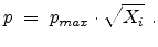
where is the atom density in the target. This model uses a constant flight
path length
and the collision partner is placed in a circular area
with the radius on a plane perpendicular to the direction of motion
with the distance
from the actual ion position. The actual amorphous
impact parameter is calculated by using the realization  from the set of
uniformly distributed random numbers
from the set of
uniformly distributed random numbers
 in the interval
according to
in the interval
according to
 |
(3.36) |
The maximum impact parameter is determined only by the target atom density:
![$\displaystyle p_{max} \;=\; \frac{1}{\sqrt[3]{N_T}} .$](img370.png) |
(3.37) |
Figure 3.11:
Monte Carlo simulation of 50 boron trajectories in crystalline
silicon using an energy of 10keV and a tilt of 7.
|
|
Figure 3.12:
Final position of 100 boron atoms implanted with 10keV into silicon.
|
|
The nuclear stopping process is simulated with the physical BCA model which is
based on the universal ZBL potential (as described in Section 3.1.2). The BCA model
contains no tunable parameters and can be applied to all materials. The elastic
two-particle scattering process is approximated by its asymptotic behavior and
the ion is placed at the closest distance to the collision partner (which is
equal to the impact parameter) before the nuclear scattering event.
The center-of-mass scattering angle is obtained from a lookup table as
a function of the reduced impact parameter  and the reduced energy
 which are defined as
 |
(3.38) |
 |
(3.39) |
Figure 3.13:
Tabulated scattering angle as a function of the scaled quantities
impact parameter and energy.
|
|
where the universal screening length (3.14) and the transformed energy
(3.6) are used.
The calculated ion trajectories presented in Fig. 3.11 show the change of
the flight direction of ions due to heavy ion-atom collisions (small impact parameter)
as well as the retention of the flight direction as ions travel along crystalline channels.
The atomic-scale distances between nuclear collision events produce continuously
plotted trajectories (every trajectory point corresponds to a single collision event).
Fig. 3.12 shows the simulated distribution of 100 boron atoms in crystalline
silicon which are implanted from the implantation window using the same implantation
conditions as for the visualized trajectories in Fig. 3.11.
The three-dimensional visualization of the tabulated scattering angle is presented
in Fig. 3.13 by using a bicubic spline interpolation. The table values of
the scattering angle are stored in a data file for 28 energy values and 17 impact
parameter values. The surface plot
 revealed
that a small impact parameter and a low energy of the ion
produces strong nuclear scattering (
revealed
that a small impact parameter and a low energy of the ion
produces strong nuclear scattering (
 ) for a binary
collision event while channeling of ions occurs at large impact parameters or at
high energies (
) for a binary
collision event while channeling of ions occurs at large impact parameters or at
high energies (
 ). The scattering angles of the ion and
of the recoil in the laboratory system are calculated from the center-of-mass
scattering angle by (3.9) and (3.10), and the transferred
energy to the primary recoil atom of a collision cascade is obtained by
(3.11).
). The scattering angles of the ion and
of the recoil in the laboratory system are calculated from the center-of-mass
scattering angle by (3.9) and (3.10), and the transferred
energy to the primary recoil atom of a collision cascade is obtained by
(3.11).
The electronic stopping process is calculated by using the Hobler model described
in Section 3.1.3. The only physical parameter required for this electronic stopping
model is the impact parameter which is determined in the BCA model when selecting
a collision partner. The model requires for every crystalline material a set of
four parameters , , , and for each ion species
(Table 3.3). In contrast to MCIMPL, where there is only one set of parameters
per ion species for one target material available (since MCIMPL was originally
just designed for the implantation into silicon), the model parameters can be
independently calibrated for each ion-target combination in MCIMPL-II. Therefore,
different crystalline material segments can be used in one simulation domain.
Due to the fact that the model implies a dependence on the charge and the mass
of the atoms of the target material, the electronic stopping power is averaged
in the case of a compound material like SiGe. The contribution of each atom
species is considered according to the stoichiometry of the material.
In addition, a special treatment is applied for multiple collisions. While the
non-local part of the electronic stopping model is considered only once, the
local contribution to the electronic stopping process is calculated once for
each binary collision which is part of the multiple collision event.
Table 3.3:
Empirical parameters for the electronic stopping process
in silicon.
| Ion species |
Charge |
Mass |
|
 |
|
|
| Boron |
5 |
11.009 |
1.75 |
0.450 |
0.050 |
0.230 |
| Nitrogen |
7 |
14.006 |
1.6861 |
0.4364 |
0.3177 |
0.1101 |
| Oxygen |
8 |
15.994 |
1.55 |
0.099 |
3.193E-5 |
0.97 |
| Fluorine |
9 |
18.998 |
0.9 |
0.6586 |
0.08 |
0.0 |
| Silicon |
14 |
27.977 |
1.4 |
0.4 |
0.12 |
0.1 |
| Phosphorus |
15 |
30.994 |
1.2674 |
0.4212 |
0.1447 |
0.0253 |
| Germanium |
32 |
72.59 |
1.15 |
0.3 |
0.3 |
0.0 |
| Arsenic |
33 |
74.92 |
1.1316 |
0.3056 |
0.2991 |
0.0243 |
| Indium |
49 |
114.82 |
1.1 |
0.3 |
0.5 |
0.0 |
| Antimony |
51 |
120.9 |
1.1 |
0.3 |
0.5 |
0.0 |
| Xenon |
54 |
131.3 |
1.1 |
0.3 |
0.5 |
0.0 |
|
The calculation of implantation induced point defects in crystalline materials is
performed with the computationally efficient modified Kinchin-Pease damage model
in combination with the Hobler recombination model as described in
Section 3.1.4. The ion species dependent parameters of the empirical
recombination model (Table 3.4) are stored in common with the parameters of
the electronic stopping model in an ASCII data file. This file contains one data
record for each combination of ion species and target material which holds all
empirical parameters including the atomic number and atomic mass of the ion species.
Table 3.4:
Recombination model parameters for different dopant
species in silicon.
| Ion species |
|
(cm) |
| Boron |
0.139 |
 |
| Phosphorus |
1.0 |
 |
| Arsenic |
2.1 |
 |
|
Figure 3.14:
Illustration of the dose dependence for boron profiles using
an energy of 20keV and a tilt of 0, simulated with the Kinchin-Pease model.
|
|
Fig. 3.14 compares simulated boron profiles for 20keV channeling implantations
in (100) silicon (shown by continuous lines) to SIMS measurements for the doses of
 ,
,  , and
, and  cm
cm . The one-dimensional profiles were
obtained with one million simulated particles using an ion beam divergence of
. The one-dimensional profiles were
obtained with one million simulated particles using an ion beam divergence of
 in the simulations. It can be observed that the shape of the
boron profiles is significantly influenced by the produced crystal damage.
The accumulation of point defects with increasing implantation dose is well
reproduced by the combined damage modeling approach based on the generation and
recombination of point defects. It should be noted that the assumption of a native
oxide film of 1nm thickness on the wafer surface is necessary to obtain a good
agreement between boron simulation results and experimental data.
in the simulations. It can be observed that the shape of the
boron profiles is significantly influenced by the produced crystal damage.
The accumulation of point defects with increasing implantation dose is well
reproduced by the combined damage modeling approach based on the generation and
recombination of point defects. It should be noted that the assumption of a native
oxide film of 1nm thickness on the wafer surface is necessary to obtain a good
agreement between boron simulation results and experimental data.
The atomic-scale simulation of ion implantation processes using a Monte Carlo
method is one of the most time-consuming computational tasks in semiconductor
process simulation. On the one hand side, dramatically shrinked geometries of
advanced devices require highly accurate simulation results by computing a
very large number of ion trajectories and, on the other hand side, applications
with higher implantation energies produce long trajectories in large-volume
simulation domains. Three speed-up methods can be employed for the trajectory
calculation in three-dimensional applications to get shorter
simulation runtimes without loosing accuracy:
- Trajectory-Split method
- Trajectory-Reuse method
- Parallelization of trajectory calculation
The simulation of ion implantation produces a statistical distribution of the
implanted dopant ions (in initial ion direction and lateral), where most of the
simulated ions come to rest at a penetration depth close to the projected range
in the target. For instance, regions with a dopant concentration of three orders
of magnitudes smaller than the maximum concentration are reached just by one
of thousand implanted ions. The statistical accuracy of simulation results
becomes even worse in regions with lower dopant concentrations, since a
reasonable simulation result includes three to five orders of the dopant
concentration. At least some implanted particles have to be counted even in
histogram cells located in peripheral regions with a very low concentration
level of dopants, since no significant information can be derived from a
histogram cell which contains only one implanted particle.
The basic idea of the Trajectory-Split method is to increase the number of ion
trajectories that end up in regions with a bad statistical representation of
dopants by splitting a particle trajectory [80,42].
The splitting of a particle produces several particles with the same physical
properties as the original particle but with a reduced weighting factor.
The increase in the number of dopants, vacancies, and interstitials caused by
a splitted particle are multiplied with the weighting factor before they are
stored in the corresponding histogram. While the simulation of a molecular ion
is performed with a weighting factor larger than one to account for statistical
identical particles of the same atom species in the molecule [81],
the weighting factor has to be below one for a splitted elemental ion to
conserve the total implantation dose. The build-up of a trajectory tree is
implemented by the full calculation of a primary trajectory and determining
of the split points along this trajectory according to various rules.
Afterwards a new trajectory is calculated from every split point up to the
end point. In crystalline materials the vibration of the lattice atoms
guarantees that two branches of a trajectory tree are not identical after
a split point despite equal initial conditions at the split point.
Figure 3.15:
Monte Carlo simulation of a boron trajectory tree
with a split depth value of 5, an energy of 10keV, and a tilt of 0
in crystalline silicon.
|
|
The effect of the Trajectory-Split method is that one implanted particle
delivers several effective ions which share the same initial part of the
trajectory. Therefore less initial ions are required to get a simulation
result with the same statistical accuracy. The sharing of parts of a trajectory
reduces the average calculation time for trajectories of effective ions.
The visualized boron trajectory tree, shown in Fig. 3.15, has a split depth
of five, which corresponds to  trajectories with a particle weight of
 . Finally, it should be noted that the Trajectory-Split method is
typically applied for crystalline materials to reduce long computation times
and to improve the statistical accuracy of doping profiles in the channeling
tail region.
. Finally, it should be noted that the Trajectory-Split method is
typically applied for crystalline materials to reduce long computation times
and to improve the statistical accuracy of doping profiles in the channeling
tail region.
The basic idea of the Trajectory-Reuse method is to use the fact that different
regions of the simulation domain behave identical with respect to the trajectory
calculation [42].
Therefore it is possible to calculate a trajectory only once and to copy it
to other regions. The copying of trajectories can be interpreted as spreading
one-dimensional simulation results over a two- or three-dimensional simulation
domain as far as possible. In terms of trajectory calculation two regions
are considered identical, if all material properties that influence the particle
motion are equal along the complete trajectory. In the case of amorphous
materials only the density and composition of the material are considered in
the simulation, while in the case of crystalline materials the trajectory is
also influenced by the damage distribution in the material.
Therefore the Trajectory-Reuse method can only be applied to amorphous
materials, because regions with an exactly identical damage distribution
along the complete trajectory are very improbable. They exist only for an
initially undamaged crystal structure.
Figure 3.16:
Illustration of the Trajectory-Reuse method for
two different materials.
|
|
Fig. 3.16 demonstrates how the Trajectory-Reuse method works for a
trench structure and for crossing the boundary between two amorphous materials
A and B. As described in Section 3.2.2 the implantation window is subdivided into
subwindows and one ion is started from each subwindow during every time step.
The Trajectory-Reuse algorithm splits a calculated trajectory which goes through
different materials into several sub-trajectories, one for each amorphous
material, and stores the obtained sub-trajectories in a list. All parts of a
calculated trajectory in crystalline materials are neglected. When the next
ion is started, the algorithm searches through the stored trajectory list.
The target material of a stored trajectory must be identical to the entrance
material of the ion and the ion energy must be less than the energy loss
along a stored trajectory. A new trajectory is calculated and
added to the trajectory list, if no suitable trajectory is available in the
list.
The Trajectory-Reuse method improves significantly the simulation speed for
three-dimensional implantation applications, since large regions of MOS
transistor structures are typically composed of amorphous materials.
Finally, it should be noted that the performance gain of this method increases
with decreasing subwindow size.
The three-dimensional Monte Carlo simulation of ion implantation requires fairly
long simulation run-times to achieve accurate simulation results in complex target
structures, which can be in the order of several days on a modern computing environment.
The simulation performance can be significantly improved by parallelization of the
trajectory calculation. Two parallelization strategies can be used in principle
for the trajectory calculation:
- Parallel computing on a cluster of workstations
- Parallel computing on a shared-memory multiprocessor system
A parallelization method based on the Message Passing Interface (MPI) was
implemented in MCIMPL [82]. The intention was to perform a
distributed simulation on a cluster of workstations which are connected over a
slow network. The simulation domain was geometrically distributed among several
workstations which have to exchange only a small amount of data during the
simulation. Due to the distribution of the memory requirement among several
workstations, small workstations could be used for three-dimensional simulations.
However, the current status of the object-oriented simulator MCIMPL-II is that
the trajectory calculation is implemented only in a sequential manner.
For future work, a powerful parallelization of the simulator can be achieved
by using OpenMP based parallel computing on a shared-memory multiprocessor
architecture [83].
The OpenMP standard provides a portable standard parallel API specifically for
programming shared-memory multiprocessor systems. This standard supports also
an incremental parallelization by adding compiler directives to the
source code. The execution of the simulation program on one multiprocessor
workstation ensures a more reliable operation for longer simulation runs
compared to a network based MPI solution. The damage accumulation during the
simulation has to be considered for parallel computing of trajectories. Only a
small error occurs, if the trajectories for all subwindows of the implantation
window are computed in parallel using the initial damage distribution of the
current time step. At the end of the time step, it has to be ensured that the
newly generated damage is updated in the shared internal data structures before
proceeding with the next time step.
After the calculation of the desired number of ion trajectories, the doping
information is stored in histogram cells aligned on an orthogonal grid. Each
histogram cell contains a certain number of implanted ions, and the doping
concentration within a cell is given by the number of ions divided by the
volume of the cell. The statistical nature of the Monte Carlo implantation
process produces a statistical fluctuation in the obtained raw cellular doping
information. In particular, three-dimensional Monte Carlo implantation results
have inherently large variances in the peripheral regions.
An advanced smoothing technique based on a Bernstein polynomial approximation
has been developed [84,85,86,14]
in order to transfer the cellular data to an unstructured destination grid
which is suitable for the subsequent process simulation step. Finite element
simulations are used in the next simulation step to imitate thermal annealing
processes which are required to activate the dopants and to eliminate the
substrate damage. On the one hand side, the postprocessing procedure performs
the necessary interpolation operation, and on the other hand side, it reduces
the statistical noise of the obtained doping and damage data.
Figure 3.17:
Illustration of the smoothing operation performed
for one point of the new unstructured grid in a two-dimensional example.
The orthogonal lines confine the cells of the internal grid. The four dashed
lines denote the unstructured grid, where the new point is marked by a
small circle. In the first step the  sample points are used to calculate
the concentration
sample points are used to calculate
the concentration  at the middle of the central grey cell.
Then the scalar product of the gradient
at the middle of the central grey cell.
Then the scalar product of the gradient
 and the
offset vector d is calculated to estimate a value for the delta
concentration.
and the
offset vector d is calculated to estimate a value for the delta
concentration.
|
|
The postprocessing procedure starts by invoking the mesh generator
DELINK [79] and passing over a point cloud in common with all
interfaces and surfaces present on the Wafer-State-Server to discretize the
doping distribution. As a result, the mesh generator produces a tetrahedral
mesh which is approximately aligned to the surface and which is fine enough to
resolve the doping profile. This mesh is handed over to the Wafer-State-Server
where the doping information is added to the points (Fig. 3.9).
Therefore, the Wafer-State-Server calls the Bernstein approximation operation
provided by the MCIMPL-II core module for each point of the new mesh.
The smoothing of the Monte Carlo result is performed by approximating the
doping concentration value for a grid point of the unstructured grid by means of
Bernstein polynomials defined in a cubical surrounding space [85].
The Bernstein polynomial
 approximates a function
of 3 variables, where
approximates a function
of 3 variables, where
 are the concentration sample points
in each dimension. The Bernstein approximation
are the concentration sample points
in each dimension. The Bernstein approximation
 is specified by
 sample points, whereby
does not run through the sample
points, but each of them affects the approximated function. The sample points
are also referred to as control points, since they enforce the progression of
the multivariate function. A critical issue is that the calculation of the
Bernstein approximation requires a reasonable information in all sample points.
In order to fulfill this requirement, the concentration value of a cell which
contains no doping information (empty cell) is determined by averaging over
the values of non-empty neighboring cells. Due to the fact that the evaluation
of the Bernstein polynomial at an arbitrary point is computationally very
expensive, the polynomial is only calculated for the middle point
sample points, whereby
does not run through the sample
points, but each of them affects the approximated function. The sample points
are also referred to as control points, since they enforce the progression of
the multivariate function. A critical issue is that the calculation of the
Bernstein approximation requires a reasonable information in all sample points.
In order to fulfill this requirement, the concentration value of a cell which
contains no doping information (empty cell) is determined by averaging over
the values of non-empty neighboring cells. Due to the fact that the evaluation
of the Bernstein polynomial at an arbitrary point is computationally very
expensive, the polynomial is only calculated for the middle point
 of the domain
 ![$ [0,1]^{3}$](img398.png) .
For that special point the Bernstein polynomial can be significantly simplified
according to the formula given in (3.40) which enables a fast
computation of the approximated value.
.
For that special point the Bernstein polynomial can be significantly simplified
according to the formula given in (3.40) which enables a fast
computation of the approximated value.
 |
(3.40) |
The drawback of this simplification method is that the obtained approximated
value is independent of the given point position somewhere in the cell. This
drawback is eliminated by also calculating the derivative of the Bernstein
polynomial at the center of the cell and modifying the approximated value
according to this local gradient as shown in Fig. 3.17.
Therefore, the concentration difference
 between the
new point and the cell middle point is calculated by the system of
equations (3.41), (3.42) and (3.43) and added to the
approximated value
at the cell middle point.
Equation (3.43) points out that it is possible to calculate the
required three partial derivatives in a fast way too.
between the
new point and the cell middle point is calculated by the system of
equations (3.41), (3.42) and (3.43) and added to the
approximated value
at the cell middle point.
Equation (3.43) points out that it is possible to calculate the
required three partial derivatives in a fast way too.
 |
(3.41) |
 |
(3.42) |
 |
(3.43) |
For the analysis of the implemented smoothing algorithm, numerical experiments
were performed with the simulator MCIMPL-II on a three-dimensional structure
equivalent to a one-dimensional problem. It is assumed that all simulated ions
are statistically independent. Fig. 3.18 shows the three-dimensional
phosphorus implantation result in a crystalline silicon substrate for
 simulated ions. The corresponding statistical
fluctuation of the phosphorus concentration as a function of the penetration
depth
simulated ions. The corresponding statistical
fluctuation of the phosphorus concentration as a function of the penetration
depth  is visualized in Fig. 3.19 for the unstructured grid. Each
sample consists of the concentration values
is visualized in Fig. 3.19 for the unstructured grid. Each
sample consists of the concentration values
 located in a horizontal plane = const. The one-dimensional doping profile
is derived by calculating the mean concentration value
located in a horizontal plane = const. The one-dimensional doping profile
is derived by calculating the mean concentration value
 for each sample.
The standard deviation
for each sample.
The standard deviation  of a sample defined by the values of
  grid
points in a plane = const is given by (3.44). The relative standard
deviation of the dopant concentration in a horizontal plane according
to (3.45) is a measure for the simulation error of three-dimensional
results compared to one-dimensional results.
grid
points in a plane = const is given by (3.44). The relative standard
deviation of the dopant concentration in a horizontal plane according
to (3.45) is a measure for the simulation error of three-dimensional
results compared to one-dimensional results.
Figure 3.18:
Smoothed result of a phosphorus Monte Carlo implantation in
silicon, using
 simulated ions, an energy of 25keV, and a dose
of cm.
simulated ions, an energy of 25keV, and a dose
of cm.
|
|
Figure 3.19:
Fluctuation of the smoothed three-dimensional dopant
distribution and the corresponding one-dimensional doping profile.
|
|
Figure 3.20:
Improvement of the simulation accuracy by the
smoothing procedure.
![\resizebox{0.85\linewidth}{!}{\rotatebox{0}{\includegraphics[clip]{figures/p-sigma}}}](img415.png) |
Fig. 3.19 depicts that the sample variance becomes minimal around the
projected range , since most of the ions come to rest there.
For the evaluation of the postprocessing improvement the ratio of the maximal
standard deviation
 within the range
 (twice the straggling at the mean projected range) of the doping profile, after
and before smoothing, can be used. As shown in Fig. 3.20,
(twice the straggling at the mean projected range) of the doping profile, after
and before smoothing, can be used. As shown in Fig. 3.20,
 within
= 22nm at = 30nm.
within
= 22nm at = 30nm.
 |
(3.46) |
The theoretical simulation error
of the Monte Carlo
method follows from the Central Limit Theorem [59]. Equation (3.46)
has been expectedly verified by simulation experiments with different .
In order to reduce
by
 , one has to increase
by a factor of 16. But as shown in Fig. 3.20, a significant improvement
of the statistical accuracy can also be achieved by sophisticated postprocessing,
in particular through the filtering effect of the Bernstein polynomials, which
eliminates high-frequency fluctuations from the original Monte Carlo data.
, one has to increase
by a factor of 16. But as shown in Fig. 3.20, a significant improvement
of the statistical accuracy can also be achieved by sophisticated postprocessing,
in particular through the filtering effect of the Bernstein polynomials, which
eliminates high-frequency fluctuations from the original Monte Carlo data.
The linear approximation of the delta concentration value
between the grid point of the unstructured grid and the cell middle point reduces
the effect of the cell discretization. The left diagram of Fig. 3.21 shows
the smoothed doping profile generated by the Bernstein approximation without
using the additional gradient-based approximation step. The internal cell
dimension of 5nm produces equal concentration values for the first two samples.
The right diagram shows the doping profile obtained by using the advanced
smoothing technique. The advanced algorithm produces a smoother and therefore
a more realistic doping profile. Longer simulation run times or worse statistics
would arise, if the cell dimension of the simulator is further reduced to enhance
the internal resolution. In contrast to that, the used smoothing
Figure 3.21:
Smoothing without (left) and with (right) linear
approximation step.
|
|
Figure 3.22:
Implantation of arsenic ions into a complex device structure
with an energy of 70keV and a dose of
 cm.
cm.
|
|
technique improves the accuracy of three-dimensional Monte Carlo implantation
results in a computationally efficient way.
Being based on random numbers, the results obtained with the Monte Carlo
technique are never exact, but rigorous in a statistical sense. Therefore, a
confidence interval can be constructed for the one-dimensional doping profile
shown in Fig. 3.19 in order to estimate the error of the mean in a plane
= const [59]. The relationship (3.46) can also be used to
estimate the number of initial ions required to obtain a specific precision
in a Monte Carlo simulation study. For the calculation of the required number
as a function of the desired maximum standard deviation
 ,
a parameter
,
a parameter  is used which takes the dopant species and the implantation
energy into account. The following formula can be used to estimate the number
for an implantation window size
is used which takes the dopant species and the implantation
energy into account. The following formula can be used to estimate the number
for an implantation window size  and a desired precision
:
and a desired precision
:
 |
(3.47) |
where
 is the investigated top surface area of
the simulation domain shown in Fig. 3.18, and the parameter
is the investigated top surface area of
the simulation domain shown in Fig. 3.18, and the parameter
 for a phosphorus implantation with an ion energy of 25keV [86].
Note that the computational effort of three-dimensional implantation applications
grows proportionally to the implantation window size in order to maintain a
certain statistical accuracy of the simulation results.
for a phosphorus implantation with an ion energy of 25keV [86].
Note that the computational effort of three-dimensional implantation applications
grows proportionally to the implantation window size in order to maintain a
certain statistical accuracy of the simulation results.
Fig. 3.22 shows the smoothed Monte Carlo implantation result. The arsenic
source/drain implantation was performed with an energy of 70keV and a dose of
 into a modern MOS transistor structure.
The simulation was carried out with 2000000 initial ions and the default
split-depth of five to demonstrate the fluctuation of the resulting dopant
distribution. It is recommended to use at least 2000000 ions/
into a modern MOS transistor structure.
The simulation was carried out with 2000000 initial ions and the default
split-depth of five to demonstrate the fluctuation of the resulting dopant
distribution. It is recommended to use at least 2000000 ions/
 ,
otherwise the simulation result is inacceptably inaccurate due to statistical
fluctuations.
,
otherwise the simulation result is inacceptably inaccurate due to statistical
fluctuations.
3.2.5 Three-Dimensional Demonstration Example
The presented simulation example explains the accomplishment of three-dimensional
implantation applications with the simulator MCIMPL-II in principle.
For complex targets it is advantageous to add the desired unstructured output
grid for the implantation result already to the input structure used for the ion
implantation simulation rather than to generate the output grid on-the-fly as
shown in Fig. 3.8. This approach allows to manually adjust the grid
refinement for a specific application. A simulation application typically
includes the following steps:
- Generation of the device geometry in the WSS format
- Addition of the unstructured grid to the geometry
- Simulation of the ion implantation step (with the option
reuse grid)
Fig. 3.23 shows the non-planar oxide mask and the unstructured grid
used in the implantation example. The two-segment geometry consisting of
silicon and oxide was generated with the three-dimensional
solid modeler LAYGRID [87].
LAYGRID reads its input from a text file which contains the geometric structure
represented by layers and polygons, and some properties of the used materials.
Each layer is defined by a two-dimensional mask and a layer thickness.
Figure 3.23:
Non-planar two-segment structure (left) and unstructured grid (right).
|
|
Figure 3.24:
Boron implantation result in the non-planar oxide mask
performed with an energy of 20keV and a dose of
 cm.
cm.
|
|
Figure 3.25:
Visualization of the boron result and the grid
lines in a geometry corner.
|
|
Figure 3.26:
Visualization of the boron result and the
tetrahedral elements which are shrinked to 40% of their original size.
|
|
The thickness is always constant for ideally planarized structures and for
non-planar layers it is necessary to define a three-dimensional surface area.
A layer mask definition contains the geometry information and material
references of all included material segments.
The resulting geometry is then written to a WSS file.
The visualized grid in Fig. 3.23 has been added to the WSS file by
the mesh generator DELINK with the box refinement method. This
method allows to control approximately the distance of the grid points in the
 and direction within a specified box-shaped container.
A finer grid resolution is used up to the expected maximum penetration depth
of the boron distribution.
Fig. 3.24 shows the implanted boron distribution in the oxide mask which
has been produced by 25 million simulated ions without using the splitting
of trajectories. In this application, the implantation window of approximately
and direction within a specified box-shaped container.
A finer grid resolution is used up to the expected maximum penetration depth
of the boron distribution.
Fig. 3.24 shows the implanted boron distribution in the oxide mask which
has been produced by 25 million simulated ions without using the splitting
of trajectories. In this application, the implantation window of approximately
 is divided into 36 subwindows which requires to
start 694445 ions per subwindow. An internal histogram resolution of 10nm
was used to discretize a cuboid region (internal simulation domain) of
the input geometry. The upper limit of the discretization cuboid is
determined by the highest position of the oxide mask surface and the lower
limit is derived by the estimated maximum penetration depth of 400nm from
the lowest oxide mask surface position.
Fig. 3.25 shows the grid lines and Fig. 3.26 the
tetrahedral elements located in the zoomed-in right upper corner on the front
side of the geomemtry. For the final boron result, 99754 grid points and
564887 tetrahedrons are used.
is divided into 36 subwindows which requires to
start 694445 ions per subwindow. An internal histogram resolution of 10nm
was used to discretize a cuboid region (internal simulation domain) of
the input geometry. The upper limit of the discretization cuboid is
determined by the highest position of the oxide mask surface and the lower
limit is derived by the estimated maximum penetration depth of 400nm from
the lowest oxide mask surface position.
Fig. 3.25 shows the grid lines and Fig. 3.26 the
tetrahedral elements located in the zoomed-in right upper corner on the front
side of the geomemtry. For the final boron result, 99754 grid points and
564887 tetrahedrons are used.
Next: 4. Doping of Group-IV-Based
Up: Dissertation Robert Wittmann
Previous: 2. Semiconductor Doping Technology
R. Wittmann: Miniaturization Problems in CMOS Technology: Investigation of Doping Profiles and Reliability
![\resizebox{0.99\linewidth}{!}{\rotatebox{0}{\includegraphics[clip]{figures/kp-frenkel-comb}}}](img336.png)
![\resizebox{0.97\linewidth}{!}{\rotatebox{0}{\includegraphics[clip]{figures/path-cylinder-comb}}}](img364.png)
![\resizebox{0.82\linewidth}{!}{\rotatebox{0}{\includegraphics[clip]{figures/traj_50}}}](img371.png)
![\resizebox{0.92\linewidth}{!}{\rotatebox{0}{\includegraphics[clip]{figures/scatter}}}](img377.png)
![\resizebox{0.9\linewidth}{!}{\rotatebox{0}{\includegraphics[clip]{figures/B_dose}}}](img385.png)
![\resizebox{0.85\linewidth}{!}{\rotatebox{0}{\includegraphics[clip]{figures/tree}}}](img388.png)
![\resizebox{0.6\linewidth}{!}{\rotatebox{0}{\includegraphics[clip]{figures/gradient}}}](img392.png)
![\resizebox{1.025\linewidth}{!}{\rotatebox{0}{\includegraphics[clip]{figures/p-result-comb}}}](img413.png)
![\resizebox{0.9\linewidth}{!}{\rotatebox{0}{\includegraphics[clip]{figures/p-fluct}}}](img414.png)
![\resizebox{0.875\linewidth}{!}{\rotatebox{0}{\includegraphics[clip]{figures/mcappl-comb}}}](img422.png)
![\resizebox{0.965\linewidth}{!}{\rotatebox{0}{\includegraphics[clip]{figures/bogen-bar}}}](img432.png)
![\resizebox{0.77\linewidth}{!}{\rotatebox{0}{\includegraphics[clip]{figures/corner-gridelem.eps}}}](img434.png)
![\resizebox{0.65\linewidth}{!}{\rotatebox{0}{\includegraphics[clip]{figures/calctraj}}}](img236.png)


![\resizebox{0.91\linewidth}{!}{\rotatebox{0}{\includegraphics[clip]{figures/b_100pt.eps}}}](img372.png)
![\resizebox{0.68\linewidth}{!}{\rotatebox{0}{\includegraphics[clip]{figures/traj-reuse}}}](img391.png)
![$\displaystyle =\; \sqrt{\frac{1}{n-1}\;\sum_{i=1}^{n} \left[C_i-\overline{C}(n)\right]^{2}} ,$](img410.png)

![\resizebox{0.92\linewidth}{!}{\rotatebox{0}{\includegraphics[clip]{figures/nograd-grad-comb}}}](img421.png)
![\resizebox{1.05\linewidth}{!}{\rotatebox{0}{\includegraphics[clip]{figures/bogen-grid-comb}}}](img431.png)
![\resizebox{0.77\linewidth}{!}{\rotatebox{0}{\includegraphics[clip]{figures/corner-gridline.eps}}}](img433.png)