Chapter 5 Fast Feature Detection for Level-Set Functions

Surface geometries originating from process TCAD simulations are often characterized by small areas with pronounced geometric variations, and large areas which are only slightly bent or even entirely flat areas. Consider, for example, the corners and side walls of a trench, respectively.

The areas with pronounced geometric variations are referred to as features. During a process TCAD simulation the wafer surface evolves in time, which dynamically changes the surface geometry during each simulation time step. Therefore, an algorithm is needed that detects where on the surface new features emerge or dissolve. Additionally, depending on the used process model strict quality requirements are imposed on the feature detection (e.g., ignoring noise in the level-set function). Geometric feature detection or extraction of 2D and 3D data sets is a widely studied field, where the surface curvature is the primary metric [26, 27, 28, 29]. In the context of level-set method, the curvatures of the zero level-set have also been used in numerous ways to gain more insights into the geometry of the surface [126, 127, 128]. Moreover, the surface curvature is of high interest in other fields of computer science, such as fluid dynamics, where the relation between surface curvature and surface tension is of interest [129]. These simulations require a high numerical accuracy of the calculated curvature values, which in turn increases the run-time. However, since in this work the surface curvature is used to indicate parts of the simulation domain that can benefit from a higher resolution the quality of the calculated curvature values is less of a concern, as long as the numerical error is not too big. Thus, the dominant metric for feature detection is the run-time.

In this chapter, a general feature detection algorithm based on the geometric properties of a discrete surface is introduced (Section 5.1). The algorithm is independent of the chosen surface representation and is used throughout the remainder of this thesis. Due to the context of this thesis in topography simulation the primarily used surface representation are level-set functions 2D feature detection is a simplified version of the 3D case, thus, the discussion focuses on the latter and the adaptations for the 2D case are presented at the end of the discussion. Furthermore, in Section 5.2 the different curvature calculation methods for implicit surfaces presented in Section 3.4, and a novel method presented in this section, are tested for their feasibility considering geometries originating from topography simulations. These geometries are then further investigated with respect to the run-times of the feature detection algorithm and are used to calibrate a numerical feature detection parameter for topography simulations.

5.1 Feature Detection

This section introduces a formal definition of which parts of a surface are considered to be a feature. To that end, the effects of minimal surfaces on the definition of a feature are discussed. Furthermore, two feature detection algorithms based on the two classes of surface classifications (i.e., surface curvature and angle between normal vectors) are introduced [22, 127].

In Section 5.1.1 a feature of a 3D surface is formally defined. Next, in Section 5.1.2 the feature detection algorithm for 3D discrete surfaces using the surface curvatures is introduced. The for this thesis developed Big Stencil method is presented in Section 5.1.3. Furthermore, it is discussed how the calculation of the Gaussian curvature can be avoided when using the Shape Operator method for feature detection and still obtain a robust detection of the features of the surface. In Section 5.1.4 a variation of the feature detection algorithm is discussed that uses the surface classification method based on the normals of the surface. Furthermore, some preliminary performance tests are discussed. Finally, in Section 5.1.5 the adaptations to the feature detection algorithm for 2D surfaces are presented.

5.1.1 Feature Definition

As already mentioned in Section 3.1.2, a minimal surface is one that has a mean curvature \(H\) of \(0\). However, the principal curvatures \(\kappa _1\) and \(\kappa _2\) might not necessarily be equal to \(0\) on each point of the surface (see Definition 3.1.14). Another way of describing minimal surfaces is the following: Minimal surfaces are surfaces on which every point on the surface is a saddle point. The plane is a trivial example of a minimal surface, however, there are several non-trivial examples. See, for example, the surfaces depicted in Figure 5.1.

For the purpose of this work it is important to distinguish parts of a surface that locally describe a minimal surface that is not a plane (e.g., a local saddle point) from an actual plane. These observations indicate that simply considering the mean curvature of a discrete surface is not sufficient to distinguish flat parts of the surface from parts that are curved. The surfaces depicted in Figure 5.1 are obviously not a plane and bend, thus, the points on these surfaces describe features of the geometry. So, a necessary and sufficient condition for a surface point to be part of a plane is \(H=K=0\), which implies that its principal curvatures also fulfill \(\kappa _1=\kappa _2=0\). Therefore, if a point on a surface only fulfills \(H=0\) and its Gaussian curvature fulfills \(K \neq 0\) it should be considered a feature.

If a point on a discrete surface is considered to be a feature and if it fulfills \(H \neq 0\) or \(K \neq 0\) the following two problems arise:

• • The curvature values calculated for a discrete surface are numerical approximations, thus, small numerical errors can cause the calculated values to deviate from an analytical plane.

• • If the discrete surface only bends slightly, e.g., has a small numerical mean curvature value, it should not be considered a feature since only sharp geometric variations lead to problems in the discretization of the surface.

Therefore, a feature can be defined as follows:

Definition 5.1.1 is similar to calculating the curvedness of a surface [131]. However, the here discussed approach of defining a feature is computationally more efficient. The curvature calculation methods for surface meshes and discrete implicit functions discussed in Chapter 3 calculate the mean and Gaussian curvature of a surface. Thus, additional computational resources have to be devoted to calculating the principal curvatures in addition to calculating the curvedness. Additionally, the in Definition 5.1.1 given description of a feature avoids calculating the Gaussian curvature if the mean curvature is already sufficient to identify a surface point as a feature.

5.1.2 Algorithm

The features of a discrete surface are detected by iterating over all surface points:

• • Point Clouds: All points of the point cloud.

• • Surface Meshes: All vertices of the surface Mesh.

• • Level-Set Functions: The grid points in the narrow band around the zero level-set.

For each surface point the absolute mean curvature \(|H|\) is calculated. If \(|H|\) is bigger than the feature threshold parameter (i.e., feature detection parameter) \(C\), then the point on the surface is considered to be a feature. Otherwise, if \(|H| < C\) the point is checked if it is part of a minimal surface by calculating the Gaussian curvature \(K\) and comparing it against \(|K| > C\). Therefore, the algorithm detects a feature when either of the following conditions is met:

\begin{align} \label {eq:featureDetection} \begin{cases} |H| > C\text {, or} \\|H| < C \text { and } |K| > C\text {.} \end {cases} \end{align} The parallelization of the feature detection algorithm is straightforward since the curvatures of each point on a discrete surface have to be calculated independently of each other. Thus, the parallel speed-up is memory-bound and limited by the quality of the used domain decomposition of the discrete surface.

5.1.3 Curvature Based Feature Detection for Level-Set Functions

In Section 3.4 three different methods of calculating the surface curvatures of an implicit surface (e.g., a level-set function) are introduced. The General Formula and Variation of Normal methods can be implemented directly as they are presented in Section 3.4. The Shape Operator method, however, requires further discussion before it can be utilized for feature detection, which is done later in this section. Furthermore, a novel way of calculating the derivatives required for the curvature calculation is presented that does not increase the stencil size but uses underutilized grid points already present in the stencil to improve accuracy.

Big Stencil

Consider that a 19 point plane stencil \(\eta _P\) is present to calculate the finite differences required to determine the mean curvature of the zero level-set (c.f., Section 3.4.1 and Figure 3.8a). There exist more accurate finite difference approximations to calculate the finite differences \(D_{x}\) and \(D_{xx}\) [132]. These finite differences require no additional grid points, thus, they do not increase the size of the finite difference stencil. They can be calculated by the following finite difference formulas

\begin{align} \tilde {D}_{x}(\phi _{i,j,k}) &\approx \frac {\phi _{i+1,j+1,k} - \phi _{i-1,j+1,k} + \phi _{i+1,j-1,k } - \phi _{i-1,j-1,k}}{{4\Delta x}}, \label {eq:BigStencilX}\\ \tilde {D}_{xx}(\phi _{i,j,k}) &\approx \frac {\splitdfrac {\phi _{i+1,j+1,k} - 2\phi _{i,j+1,k} + \phi _{i-1,j+1,k} + \phi _{i+1,j,k}-2\phi _{i,j,k} } {+ \phi _{i-1,j,k} + \phi _{i+1,j-1,k} - 2\phi _{i,j-1,k} + \phi _{i-1,j-1,k}}}{3\Delta x^2}. \label {eq:BigStencilXX} \end{align} When the mean curvature is calculated using Equation 3.21 utilizing the finite difference approximations \(D_{xy}\), \(\tilde {D}_{x}\), and \(\tilde {D}_{xx}\), it is henceforth referred to as the Big Stencil method. The here suggested method uses the same finite difference stencil as the General Formula method. However, it utilizes more information of the level-set function (e.g., more \(\phi \)-values) to calculate the derivatives required in Equation 3.21. Therefore, the numerical accuracy of the calculated mean curvature values is improved. The Gaussian curvature can be calculated by using the more accurate finite difference approximations and Equation 3.22. Therefore, no additional calculations are required when using this method for feature detection.

Addendum Shape Operator

The Shape Operator method uses the trace of the Hessian to calculate the mean curvature of the discrete surface. By only requiring the trace this method can be calculated with a 7-point star stencil \(\eta _S\) (see Section 3.4.1), however, calculating the Gaussian curvature still requires a plane stencil \(\eta _P\). That larger stencil \(\eta _P\) would negate the performance gains achieved through the smaller stencil and fewer finite differences that have to be evaluated. Therefore, a different strategy to determine if a surface point is part of a minimal surface is desired. This can be achieved by utilizing the fact that the value of the mean curvature is expressed by half the trace of the Hessian. Thus, conditions of the feature detection algorithm (see Equation 5.1) are simultaneously checked if

\begin{align} \label {eq:MinSurfShape} |D_{xx}(\phi _{i,j,k})| + |D_{yy}(\phi _{i,j,k})| + |D_{zz}(\phi _{i,j,k})| > 2C. \end{align} Let the grid point \((i,j,k)\) be part of a minimal surface that is not a plane, so \(H=0\) and without loss of generality

\begin{align} -D_{yy}(\phi _{i,j,k}) = D_{xx}(\phi _{i,j,k}) + D_{zz}(\phi _{i,j,k}) \neq 0. \end{align} Thus, \(|D_{yy}(\phi _{i,j,k})| \neq 0\) and Equation 5.4 holds for points on a minimal surface that describe a feature of the zero level-set.

Nonetheless, it is possible that each element in the trace of the Hessian is equal to \(0\) when a point on a minimal surface that is not a plane is investigated. However, this case can be ignored considering the following deliberations. If all second-order derivatives of the trace are \(0\), then the basis in which the shape operator in the point \(\mathbf {x}\) is expressed has a specific form. For example, let \(\mathbf {x}\) be the saddle point of a hyperbolic paraboloid parametrized by \((x^2-y^2) - (x-y)^2=z\). When the basis vectors spanning the tangent plane of the shape operator in \(\mathbf {x}\), point in a \(45\) degree angle between the cartesian coordinate axes \(x\) and \(y\), then the second-order derivatives along these basis vectors are \(0\) since the curves are straight lines (see Figure 5.2).

However, this implies that the basis of the shape operator in the adjacent points to \(\mathbf {x}\) has to be different, thus, the trace of the Hessian in these adjacent points does not contain only zero entries.

The Shape Operator method is an often neglected method of calculating the mean curvature of a level-set function. Its numerical accuracy is highly dependent on the numerical accuracy of the signed distance function, which in performance oriented applications is only first-order accurate (see Equation 4.13). However, in Section 5.2.3 it is shown that the numerical accuracy is high enough to use this method for feature detection.

5.1.4 Surface Normal Based Feature Detection

As mentioned in Section 3.5, when considering level-set functions the angle between the surface normal vectors can be used for surface classification. To that end, the definition of a feature (see Definition 5.1.1) has to be adapted.

This method intrinsically handles minimal surfaces since it approximates the angle between the normal vector of a parametrized curve and the central normal vector in the direction of the maximum curvature \(\kappa _1\) and not the mean curvature.

Algorithm Adaptation

The algorithm presented in Section 5.1.2 must be adapted to work with angle features. Instead of calculating the curvatures in each point on the surface, the surface normal in each surface point is calculated. Afterwards, a box stencil is moved over each surface point. Each point in the box stencil is checked if it is a surface point, when this point is a surface point the angle \(\alpha \) between the central normal and the normal of the surface point is calculated, and is checked if \(\alpha < C_{angle}\). If \(\alpha > C_{angle}\) the central point is marked as a feature and the box stencil is moved to the next surface point, otherwise the next point in the box stencil is checked.

Run-Time Evaluation of Surface Normal Based Feature Detection

The primary drawbacks of a surface normal based feature detection on level-set functions are discussed here. Depending on the position of a surface normal on the surface it is possible that the angle between the central normal and an adjacent normal is greater than the parameter \(C_{angle}\) although the central surface normal is not part of a feature. Figure 5.3 shows an illustration of such a problem.

The point \(\mathbf {p}_1\) would be flagged as a feature even though it is part of a plane.

Furthermore, the computational performance (See Section 5.2) of the surface normal and curvature based feature detection are experimentally compared. In what follows, the studies have been performed on a trench geometry shown in Figure 5.4.

The run-times and speedup of the curvature based feature detection algorithm using the General Formula, the Shape Operator method to approximate the surface curvature, and the surface normal based feature detection algorithms presented in Section 5.1 are investigated. The feature detection parameters \(C\) and \(C_{angle}\) have been chosen in such a way that they flag the same amount of grid points as features. Figure 5.5 shows the benchmarks executed on Workstation 2.

The results show that the performance of the surface normal based feature detection is far worse compared to using the surface curvatures. The additional drawback of potentially flagging more surface points than needed yields the conclusion that surface normal based feature detection is the vastly inferior choice to detect features of a level-set function compared to feature detection based on surface curvature.

5.1.5 2D Feature Detection

Feature detection on 2D surfaces is a simplified version of the feature detection algorithm presented in Section 5.1.2. The definition of a feature (see Definition 5.1.1) also holds for 2D surfaces, when the term mean curvature is substituted by curvature (i.e., \(\kappa \)). Furthermore, in the 2D case the calculation of the Gaussian curvature and discussion about minimal surfaces is immaterial, since minimal surfaces only occur in 3D. Thus, the algorithm presented in Section 5.1.2 is easily adapted for 2D discrete surfaces. In this case, the algorithm simplifies to calculating the absolute curvature \(|\kappa |\) and comparing it to the feature threshold parameter \(C\).

Surface normal based feature detection can also be used on 2D surfaces, by modifying the box stencil which only consists of 9 grid points in 2D.

5.2 Comparison and Evaluation

The simulation results presented in this section have been generated with ViennaLS and where executed on a single node of VSC4 (see Section 4.6.3).

Hierarchical Run-Length Encoding

ViennaLS uses a Hierarchical Run-Length Encoding (HRLE) data structure to store the level-set function. The HRLE data structure only stores the narrow band around the zero level-set up to a predetermined thickness (see Section 2.3) [133]. This is achieved through a segmentation of the coordinate directions. This data structure naturally lends itself to be used in a level-set framework based on the sparse field approach [114].

Parallelization Strategy

Parallelization in ViennaLS is achieved through a domain decomposition approach that splits the entire simulation domain into subdomains. The domain is split along a coordinate axis in such a way that approximately the same amount of grid points are present in each subdomain [134].

5.2.1 Geometries and Mean Curvature Values

The applicability of the curvature calculation methods presented in Section 3.4 and the newly developed Big Stencil method for the feature detection algorithm presented in Section 5.1.2 is evaluated on several test geometries:

• 1. Sphere

• 2. Stacked nanosheet FET [12]

• 3. Selectively grown epitaxial crystal [87]

Sphere

In case of the sphere the mean curvature can be analytically calculated and compared to numerical approximations. A sphere with radius \(r\) has an analytical mean curvature of \(1/r\). Furthermore, every time step in a level-set based simulation is a numerical approximation which introduces small numerical errors into the discretization of the surface. Thus, to compare the analytical mean curvature values of the sphere to values calculated during a simulation workflow, the sphere has been subjected to a velocity field. By way of example the here considered sphere is initialized with a radius of \(15\), and subsequently subjected to a constant velocity field with a velocity of \(-1\) for \(5\) time units. This results in a sphere that should have an analytical radius of \(10\), and thus, a mean curvature \(H\) of \(0.1\). A first-order Engquist Osher scheme is used to solve the level-set equation (see Section 4.1.1). The distribution of the calculated mean curvature values of all points on the zero level-set, for the Big Stencil and the methods discussed in Section 3.4, is shown in Figure 5.6. Due to the numerical errors introduced by the discretization of the level-set function, the distance to the center of the sphere from all points on the zero level-set is between \(9.9\) and \(9.6\), with an average distance of \(9.7\). The smaller radius compared to the analytical sphere is explained by a loss in volume originating from the discretization into the regular grid. Thus, the calculated mean curvature values are distributed around the analytical mean curvature of a sphere with radius \(9.7\), which is indicated by the black line in Figure 5.6.

The mean curvature values computed with the General Formula and the Variation of Normal methods do not significantly differ from each other. The mean curvature values calculated with the Shape Operator method deviate the most from the analytical solution. However, this is expected since the star stencil uses fewer grid points, thus the numerical error of the discretization is more pronounced, as discussed in Section 5.1.3. The Big Stencil method produces the best match with the expected mean curvature values from the analytical solution. These investigations show that the mean curvature calculation methods, except for the Big Stencil method, tend to overestimate the mean curvature of the sphere. Furthermore, the Shape Operator method overestimates the mean curvature values by up to \(75\%\). However, the empirical analysis presented in Section 5.2.3 shows that this error does not disqualify the Shape Operator method from being used for the purpose of feature detection.

Stacked Nanosheet FET

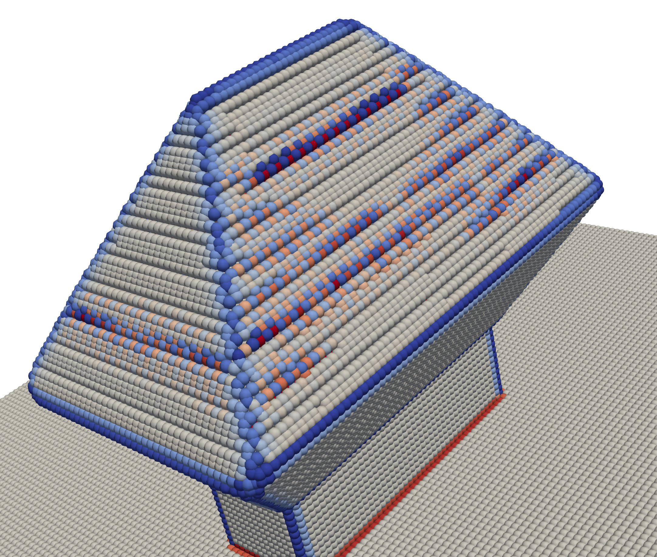
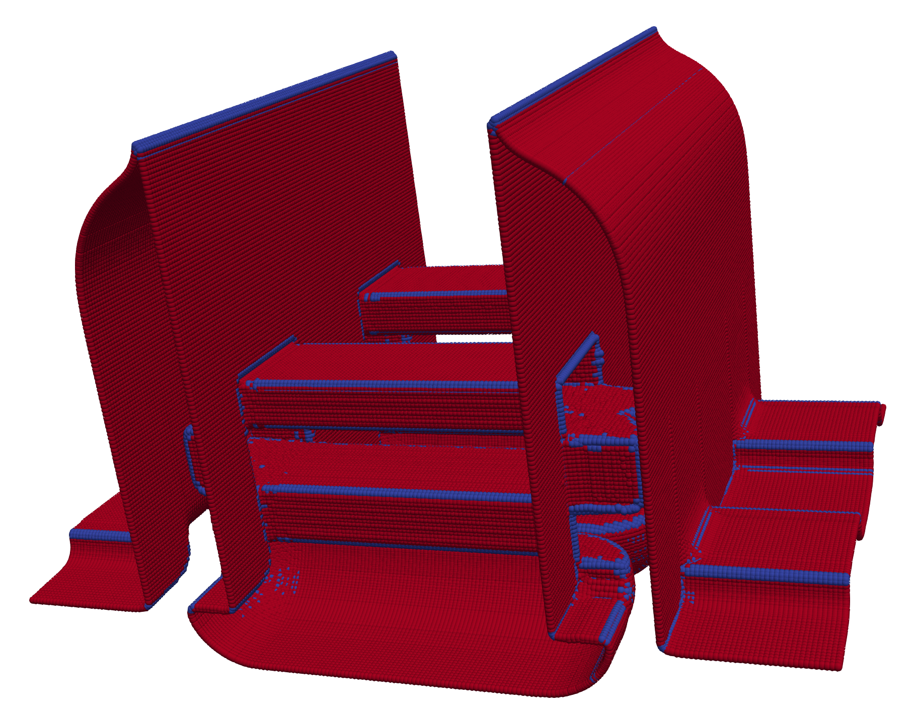
The first geometry originating form a topography simulation workflow is a stacked nanosheet FET. As discussed in Section 4.3, different materials are represented by their individual level-set functions, which are combined through layer wrapping to represent the topography of the semiconductor device. Therefore, it is sufficient to only investigate certain material layers, since the features of the underlying layers are already captured in the upper layer. Figure 5.7 shows two representative material layers (layer 3 and layer 5) after the 24th process step of a stacked nanosheet FET fabrication simulation (see Table II of [12]): the surfaces are the result of several processing steps, which have undergone considerable geometric changes due to the employed process models. For all the above-mentioned processing steps a first-order Engquist Osher scheme is used to solve the level-set equation. In Figure 5.8 the distribution of the absolute mean curvatures of layers 3 and 5 are shown.

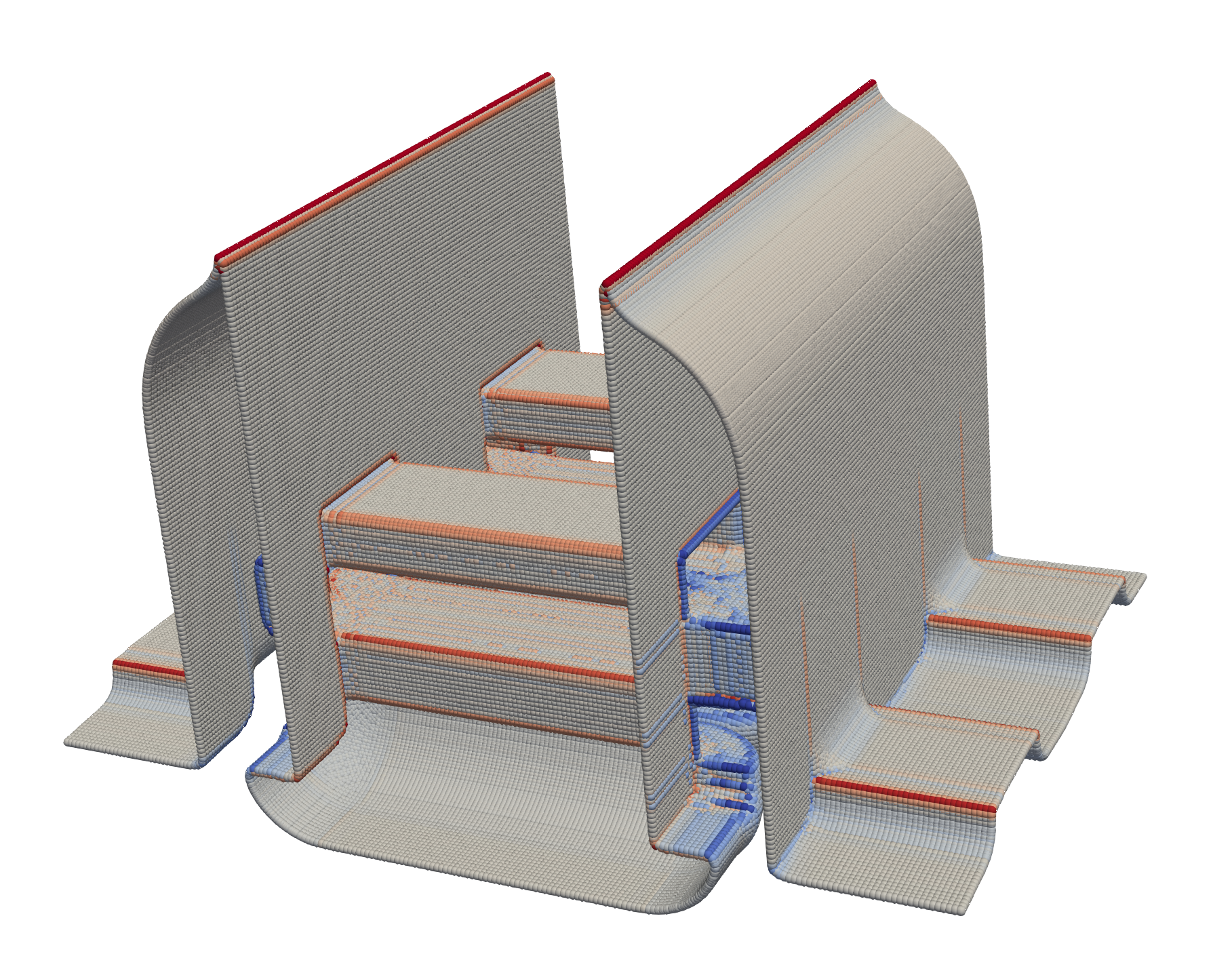
A similar behavior of the calculated mean curvature values as for the sphere can be identified. Specifically, the mean curvature values calculated with the Shape Operator method overestimate the mean curvature more than the other methods. About 96% of the calculated absolute mean curvature values fall in the interval between \(0.0\) and \(0.5\). This illustrates that most of the geometry is flat or only slightly bent, without many sharp features.

Selectively Grown Epitaxial Crystal

The second considered geometry of a topography simulation workflow is a heteroepitaxially grown \(\text {SiGe}\) crystal on a \(\text {Si}\) fin. These crystals are fabricated using strongly anisotropic processing techniques which are a common fabrication steps for non-planar semiconductor device geometries (e.g., FinFETs) [135]. The simulation of such processes result in non-convex Hamiltonians. In Section 4.1.1 the Lax-Friedrichs scheme is discussed. It is required to solve the level-set equation when simulating crystallographic orientation-dependent growth. Furthermore, the process model depends upon special interpolation schemes to calculate the velocities for all points on the zero level-set [136]. The selective epitaxial growth (SEG) of the \(\text {SiGe}\) crystal is characterized by crystal facets (i.e., the planes formed by the different growth characteristics depending on the crystallographic planes). The resulting device topographies contain areas with high-curvatures and essentially flat areas [137]. Simulating such processes results in level-set functions with sharp corners that have to be maintained during the simulation of the growth process.

Figure 5.9 depicts the \(\text {SiGe}\) material layer of the simulated crystal surface, and Figure 5.10 shows the distribution of the calculated absolute mean curvature values.

Comparing the calculated mean curvature values of Figure 5.9a and Figure 5.9b shows that there is slight noise on crystalline facets when using the General Formula method. The noise is introduced by the numerical methods used to solve the process model (e.g., the Lax-Friedrichs scheme and the interpolation of the velocity values). However, the mean curvature values calculated with the Big Stencil method shown in Figure 5.9b are only marginally affected by the noise in the level-set function. The superior results achieved with the Big Stencil method concerning the noise in the level-set function is explained by the additional grid points used to approximate the second-order derivatives: As discussed in Section 3.4.2 the trace of the Hessian of the level-set function contains all information needed to calculate the mean curvature. Thus, increasing the numerical accuracy of the second order derivatives in the same direction (i.e., the elements of the trace of the Hessian) increases the accuracy of the calculated mean curvature. Figure 5.10 supports the above observations since most of the absolute mean curvature values are smaller than \(2\) and most of them are close to \(0\), compared to the other three methods.

5.2.2 Parameter Study

In the previous section the calculated mean curvature values of several geometries originating from process TCAD simulations have been investigated. The feature detection algorithm presented in Section 5.1.2 requires a feature threshold parameter \(C\). Thus, to obtain such a parameter for the investigated topographies a parameter study is conducted. The parameter search starts with a (for this case appropriate) value of \(0.01\) for the feature detection parameter \(C\) up to \(1/\Delta x\) with a step length of \(0.01\). \(1/\Delta x\) is chosen as the maximum value, since it is the maximal absolute curvature a level-set function with a given grid resolution of \(\Delta x\) can describe (see Section 3.4). \(0.01\) is chosen as the minimum value as smaller values tend to flag nearly the entire surface as a feature. Figure 5.11 shows the different feature detection parameters \(C\) compared to the surface points detected as features for the two representative material layers of the stacked nanosheet FET.

The observations from the previous section still hold, thus, the Shape Operator identifies more surface points as features than the other methods. However, as long as the additional grid points which are detected as features are still adjacent to other features of the geometry they can be ignored. This suggests that the Shape Operator method is still able to reliably detect features of the zero level-set. The other three methods identify approximately the same number of surface points as features with only minor deviations.

The graphs depicted in Figure 5.11 indicate that the feature detection parameter \(C\) for the here considered representative topographies should be chosen between \(0.1\) and \(1.0\): If the feature detection parameter is larger than \(1.0\) almost no grid points are detected as features leading to less and less features being identified. On the other hand if the feature detection parameter is chosen smaller than \(0.1\) it is possible that nearly all surface points are detected as features. These deliberations and Figure 5.8 suggest that a feature detection parameter of \(C = 0.5\) identifies most features and simultaneously avoids capturing only slightly bent parts of the zero level-set.

Figure 5.12 depicts the same parameter search for the heteroepitaxially grown \(\text {SiGe}\) crystal surface as for the stacked nanosheet FET.

The Big Stencil method identifies far fewer grid points as features in the range of \(0.2\) and \(1.1\) than the other three methods, which contrasts the behavior of the feature detection parameter observed for the stacked nanosheet FET. As argued in Section 5.2.1 the lower amount of grid points detected as features stems from the higher accuracy of the Big Stencil method, which enables it to ignore the noise in the crystal facets. At a feature detection parameter of \(C=1.1\) (see Figure 5.12) the amount of grid points detected as features between the General Formula, Variation of Normal, and Big Stencil equalizes. However, as previously discussed this is a relatively high value (see the distribution of the mean curvature values in Figure 5.8 and Figure 5.10) for the feature detection parameter, which can lead the feature detection to miss important features of the investigated geometry. The amount of grid points detected as features is constant between the feature threshold parameters \(0.4\) and \(1.1\) when using the Big Stencil method. Thus, \(C = 0.5\) is a sensible choice for the feature detection parameter when the Big Stencil method is used to calculate the curvatures of the \(\text {SiGe}\) crystal.

5.2.3 Empirical Evaluation

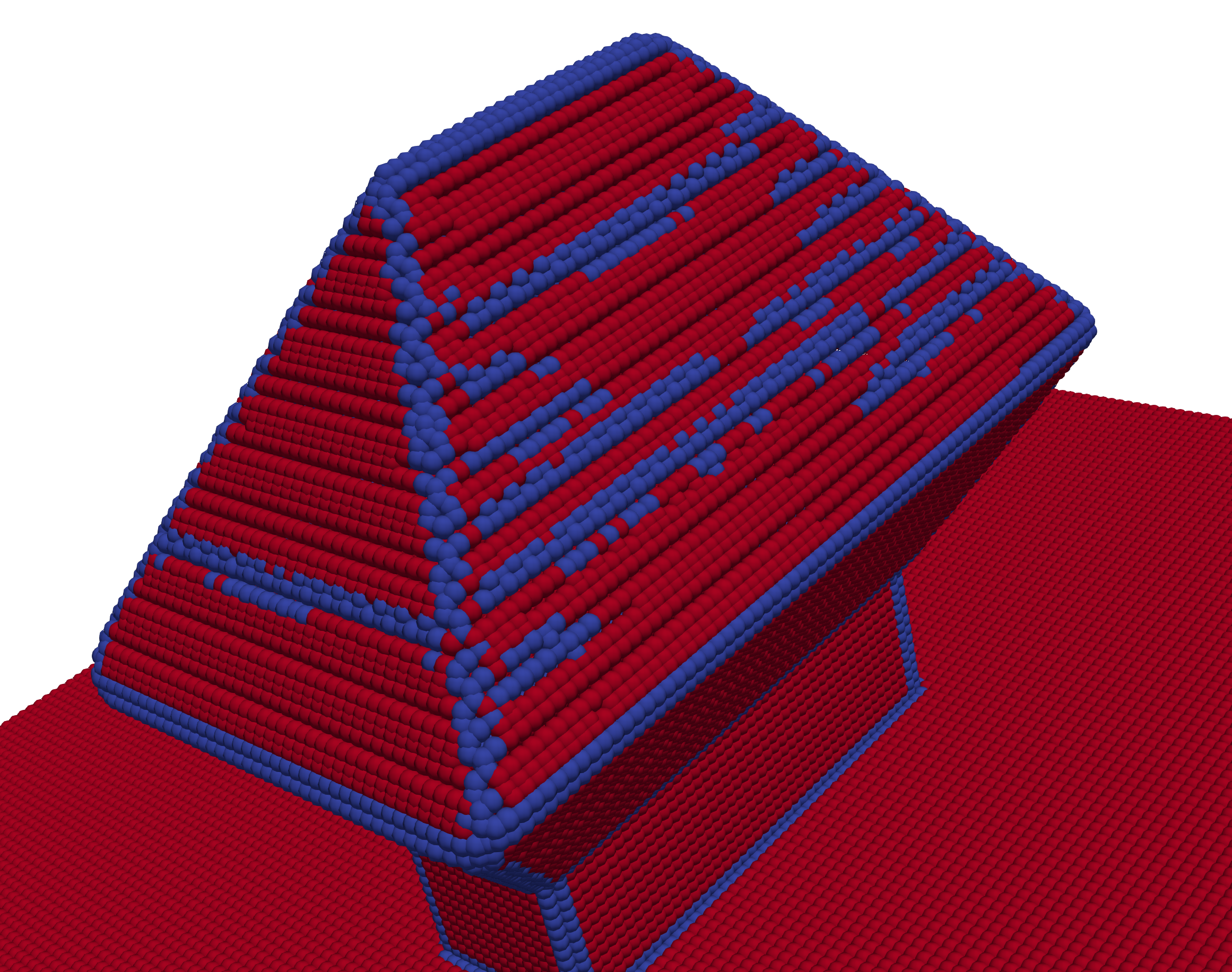
Here, the feature detection algorithm presented in Section 5.1.2 combined with the identified feature detection parameter C (see Section 5.2.2) are evaluated for their feasibility to detect features on geometries originating from process TCAD simulations. Figure 5.13 depicts the features detected by the feature detection algorithm using the Shape Operator and the Big Stencil methods on the topography of a stacked nanosheet FET.

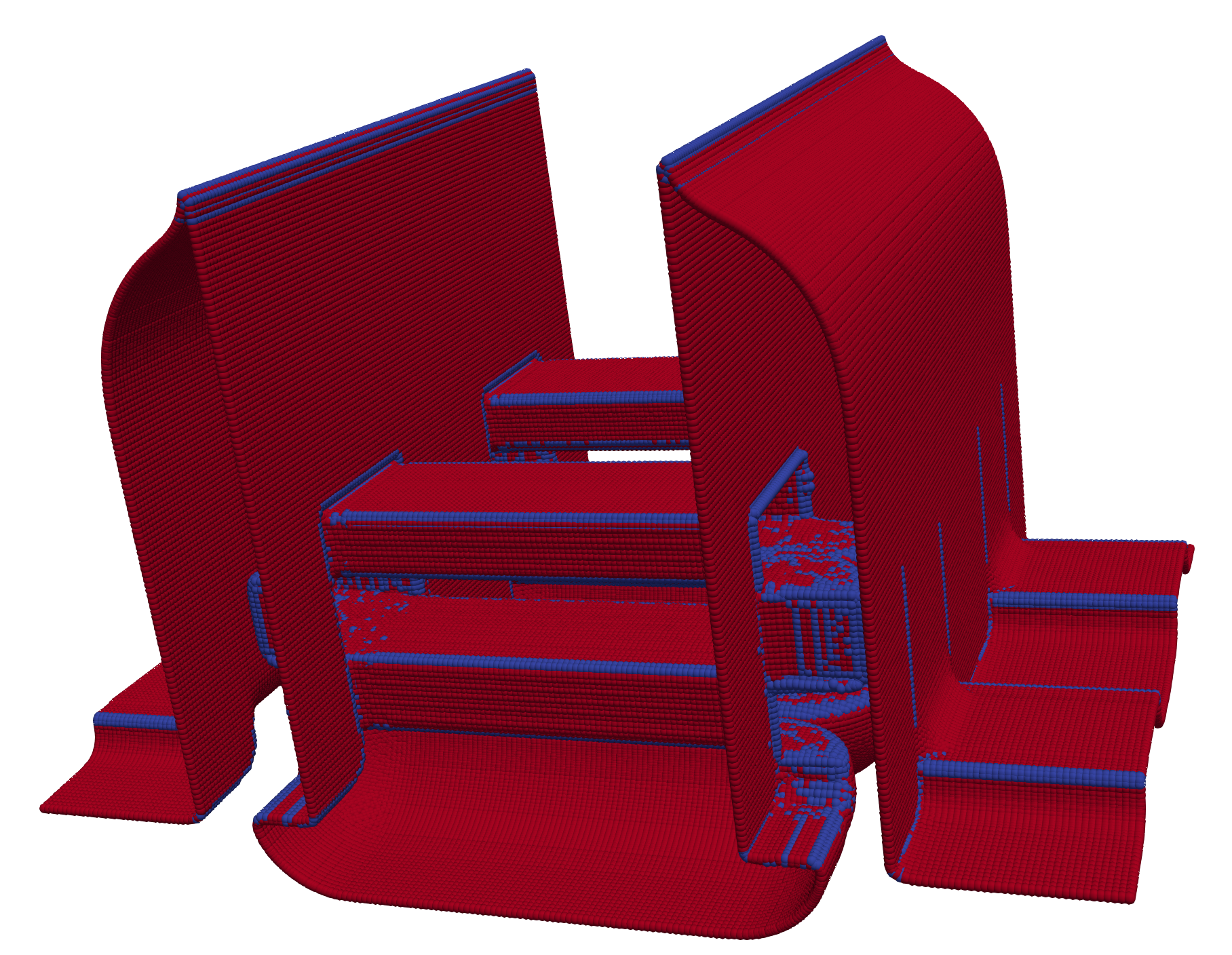
As already suggested by the results in Section 5.2.2, the Variation of Normal and General Formula method detect similar features to the other two methods. Furthermore, Figure. 5.13 confirms that a feature detection parameter of \(0.5\) is well suited to distinguish features from flat parts.

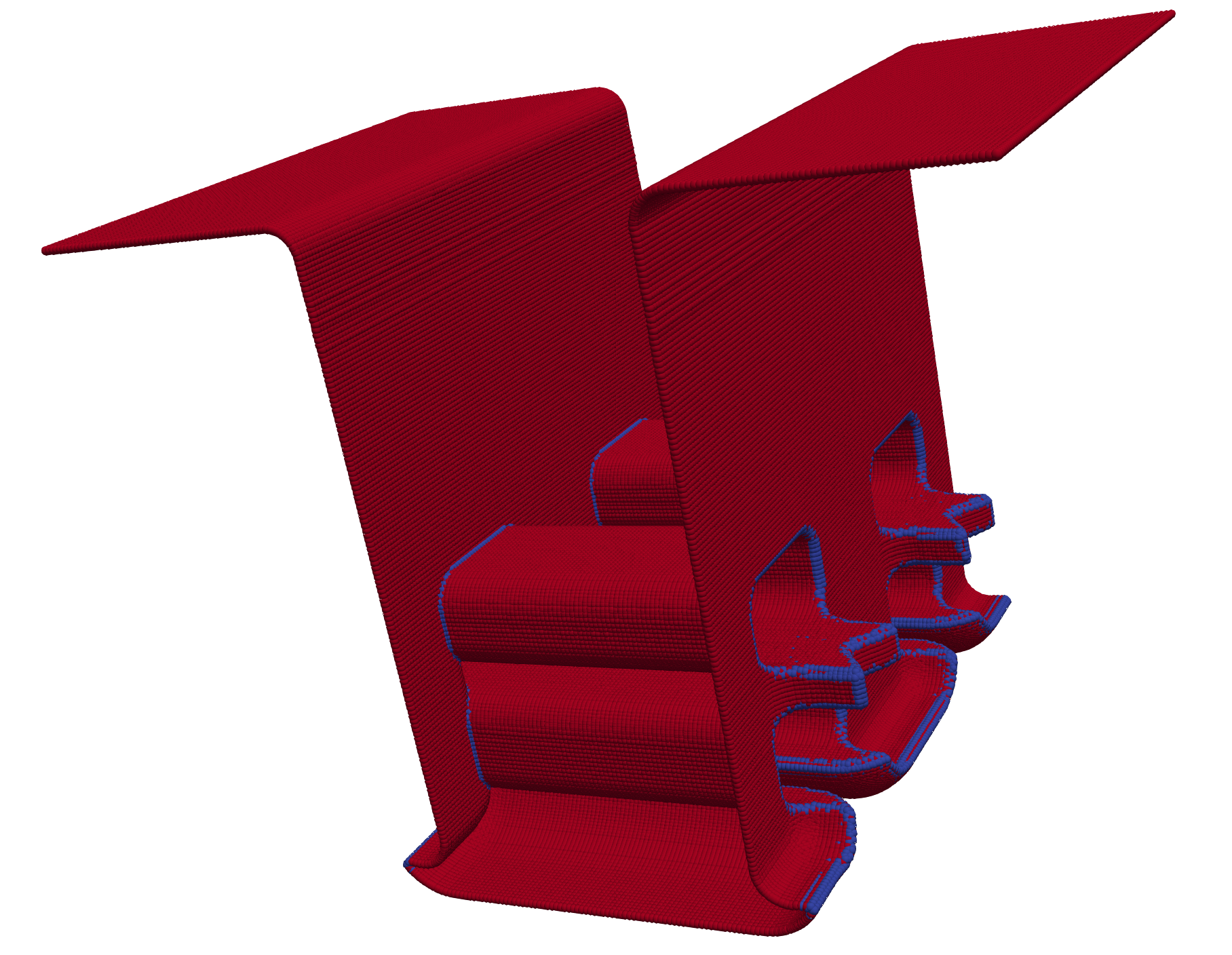
In Section 5.2.2 a feature detection parameter of \(1.1\) is suggested for the \(\text {SiGe}\) crystal, the results of the feature detection using this parameter are shown in Figure 5.14.

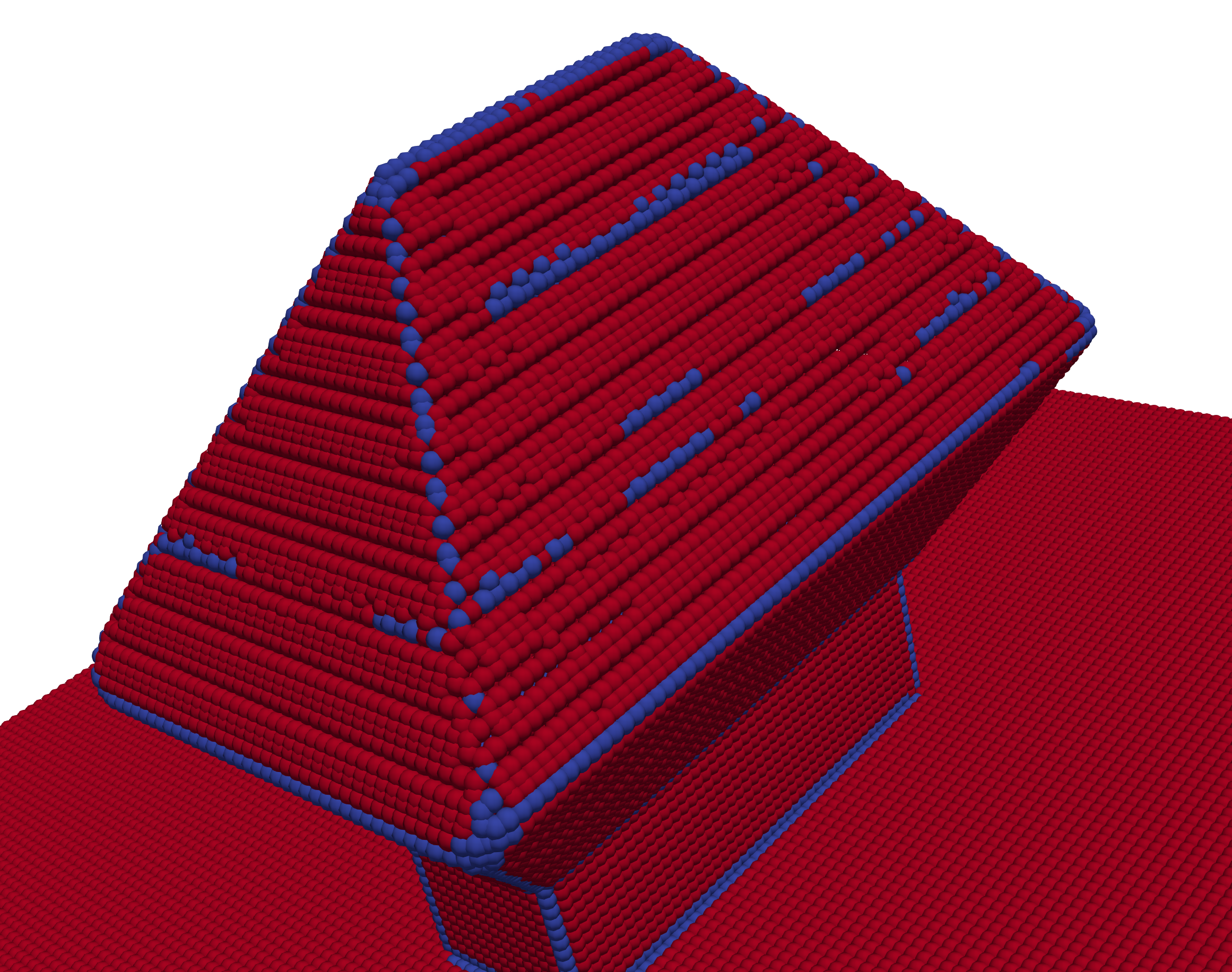
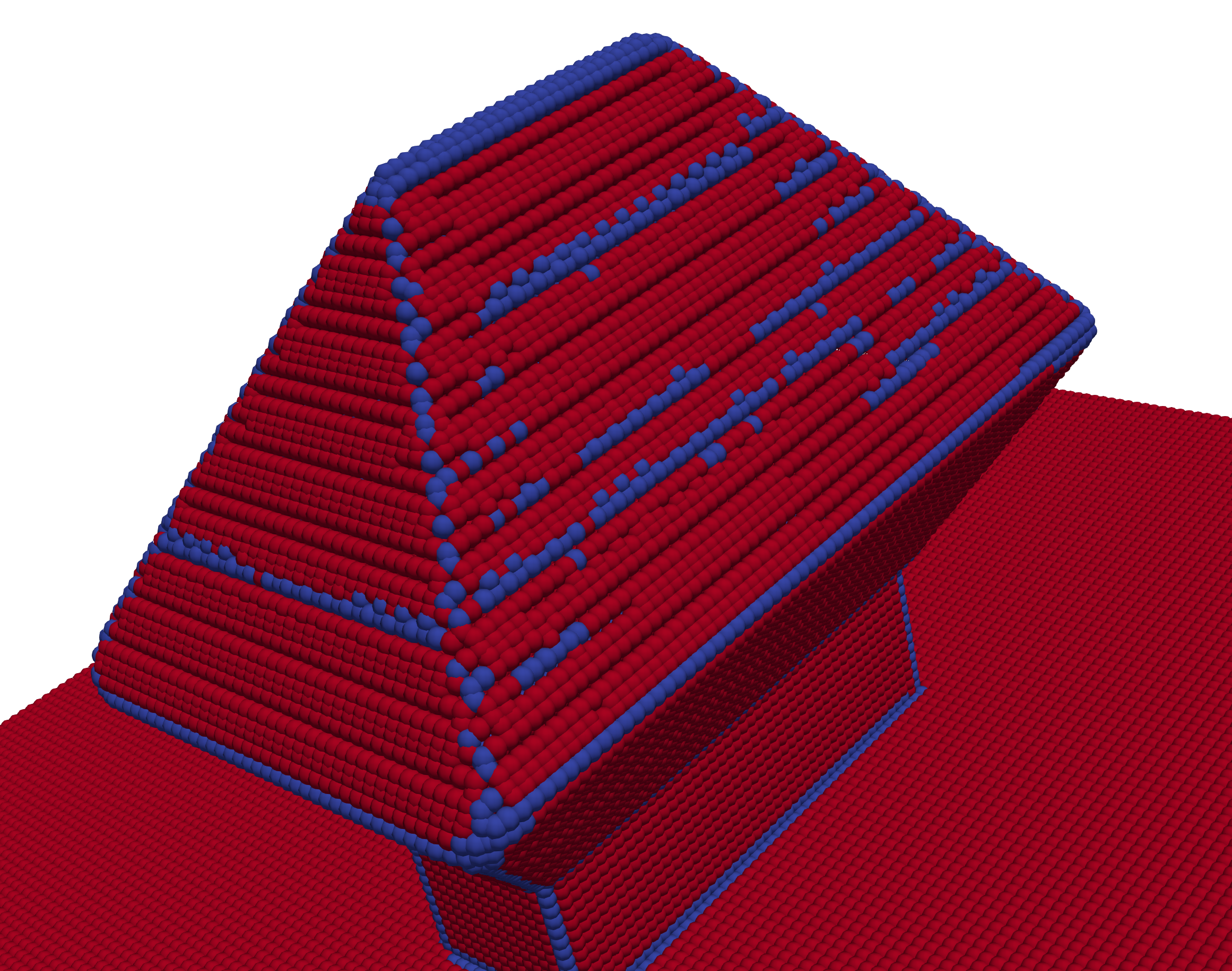
Figure 5.12 shows that all curvature calculation methods detect a similar amount of grid points as features with a feature threshold parameter of \(C=1.1\). However, when consulting Figure 5.14, it is evident, that the features detected with this feature threshold parameter are inadequate, since on the one hand points on the crystal facets are detected as features and on the other hand points at the edges of the crystal are not. The falsely detected features at the crystal facets are a consequence of noise introduced into the level-set function by the process model. Reevaluating Figure 5.12 with the above deliberations in mind, it has to be concluded that the General Formula, Shape Operator, and Variation of Normal methods are not suited for feature detection in this scenario. Nonetheless, the results generated with the Big Stencil method still appear promising, since the higher quality of the curvature calculation allows this method to ignore the noise on the crystal facets. Therefore, the results reported in Figure 5.12 for the Big Stencil method have to be reassessed: These results show that the amount of grid points detected as features stays nearly constant between a feature detection parameters of \(0.5\) and \(1.0\). Thus, a feature detection parameter of \(0.5\) is considered for the \(\text {SiGe}\) crystal, the feature detection results for the General Formula, and Big Stencil method with this feature detection parameter are shown in Figure 5.15. The results obtained with the Shape Operator, and Variation of Normal method are omitted since they are similar to the results of the General Formula method. The detected features of the \(\text {SiGe}\) crystal shown in Figure 5.15b illustrates that the Big Stencil method achieves an adequate feature detection of the \(\text {SiGe}\) crystal using a feature detection parameter of \(0.5\).

5.2.4 Parallel Run-Time and Speedup

The average performance (run-time and parallel speedup) of the feature detection algorithm applied to the geometries introduced in Section 5.2.1 is tested in this section. All four discussed curvature calculation methods are evaluated. In all three run-time tests (see Figure 5.16, Figure 5.17, and Figure 5.18) the fastest curvature calculation method is the Shape Operator method, while the other three methods have a comparable performance.

The speedup shown in Figure 5.16b illustrates the best case scenario. In light of the convexity of the sphere the domain decomposition algorithm is able to create subdomains with a very similar number of surface points. Thus, this speedup should not be expected from the more complex geometries originating from process TCAD simulations. Furthermore, the run-time and the speedup can differ due to load balancing issues, which can be observed by comparing Figure 5.17 and Figure 5.18 to Figure 5.16. In these examples the domain decomposition splits the narrow band into roughly equally sized subdomains, considering the entire grid, however, the number of surface points is not equal in each subdomain. Another issue leading to the worse speedup for the considered process TCAD geometries is the fact that feature detection (i.e., curvature calculation) is memory bound since the primary effort is the movement of the finite difference stencil over the grid.

The results presented in this section support the considerations in the previous section. Since the Big Stencil method does not result in a considerable increase in run-time compared to the General Formula and Variation of Normal methods it should be the primary choice for complex process models with noise. However, if the process model is simple and the primary concern is performance the Shape Operator method is the better choice.

5.3 Summary

In this chapter, the surface classification methods presented in Chapter 3 for the surface representations from Chapter 2 have been used to formulate a feature detection algorithm for topography simulation. Furthermore, a novel way to calculate the surface curvature using the general formula for implicit surfaces has been developed. The performance of the algorithm on 3D level-set functions with all discussed methods of calculating the curvatures has been investigated. In the course of these investigations two methods for curvature calculation of a level-set functions stood out.

The Big Stencil method displayed the highest numerical accuracy of the calculated curvature values. Furthermore, the Big Stencil method is less affected by noise in the level-set function introduced by certain process models, which has been demonstrated with the noise introduced by crystallographic orientation-dependent velocity fields. These improvements have been achieved without increasing the size of the finite difference stencil that is used for curvature calculation compared to the General Formula or Variation of Normal methods.

The Shape Operator method requires the smallest finite difference stencil to approximate the mean curvature of the level-set function. Moreover, when using the Shape Operator method the calculation of the Gaussian curvature can be avoided to check if a point on the zero level-set is part of a minimal surface, which makes this method the best performing method with respect to computational effort. However, the Shape Operator method has the lowest numerical accuracy of the investigated curvature calculation methods. Nonetheless, this does not preclude it from being utilized for feature detection as demonstrated in Section 5.2.3.

In summary, the insights obtained from the research in this chapter are: If run-time is the most important aspect for the feature detection the Shape Operator method is the preferred method to calculate the curvatures of the level-set function. On the other hand, if accuracy is the most important aspect or if there is slight noise in the level-set function, then the Big Stencil method should be used. Due to the Big Stencil methods higher numerical accuracy and similar performance to the General Formula and Variation of Normal methods. Furthermore, a parameter search for the feature detection parameter \(C\) for process TCAD simulations has been performed which resulted in a feature detection parameter of \(0.5\) for all presented methods.