Chapter 2 Surface Representations

Many problems in engineering investigate the properties or deformation of surfaces. For example, the change of the position of a surface when a physical process deforms it, on what parts of a surface materials accumulate, or how much of the surface area is exposed to a particle source [33, 34, 35]; the interaction at the interfaces of different liquids, gasses, and solid boundaries during a multiphase flow  [36, 37]; or the detection of objects in the vicinity of a laser scanner, that creates real time scans of the area around the scanner [38, 39, 40].

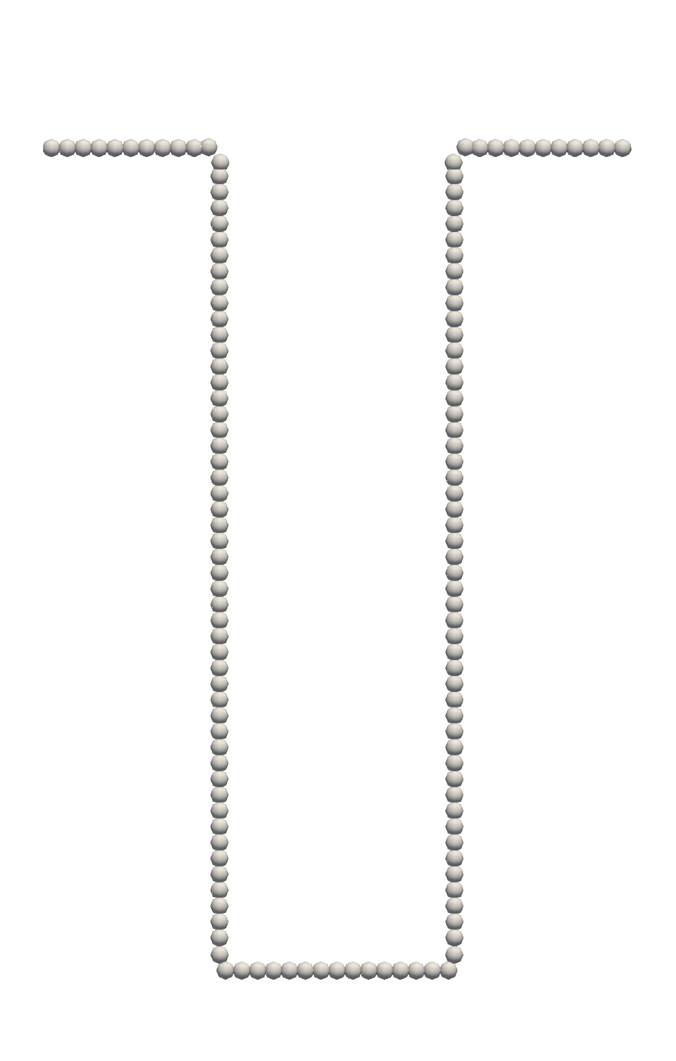
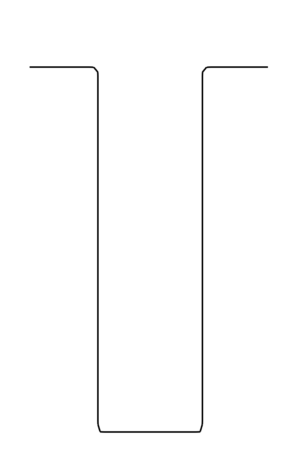
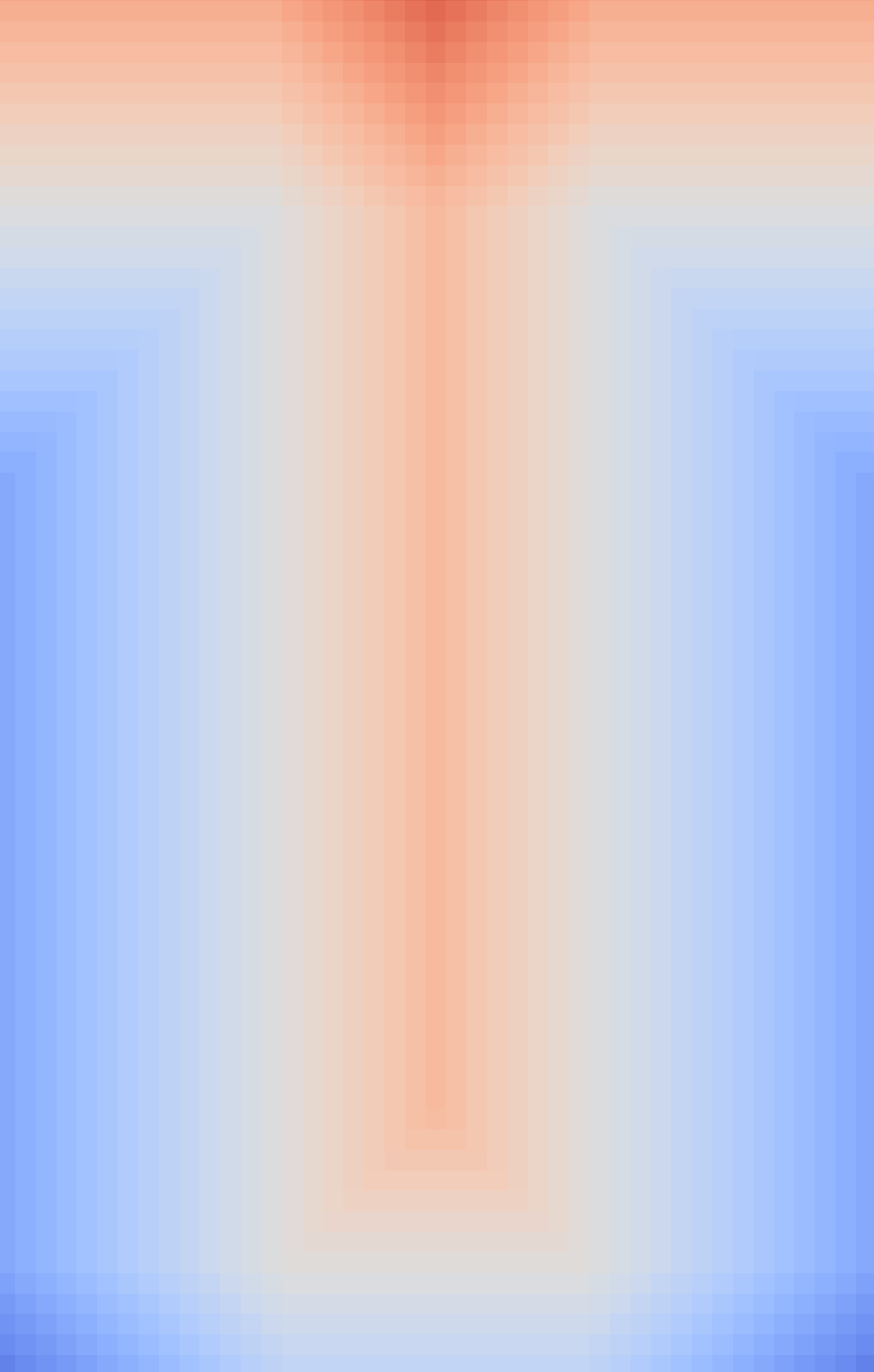
For many of these aforementioned engineering problems mathematical models exist that offer solution strategies. One fundamental aspect required to solve these engineering problems is the representation of the investigated surfaces. Most surfaces originating from real world geometries that are used in engineering applications are arbitrary, and thus, do not have a readily available differentiable mathematical description. Thus, the surfaces that describe these geometries have to be discretized to numerically apply these mathematical models. An example of three surface representations (i.e., point clouds, surface meshes, and implicit surfaces) used in this work, are shown in Figure 2.1.

Furthermore, some surface representations offer certain advantages depending on the mathematical models used in a simulation. Certain surface flux calculations use an explicit surface representations [18], since there exist powerful and performant algorithms to accomplish these tasks [41]. On the other hand, the merging of two different surfaces is better handled with an implicit surface representation [17].

In this chapter the discrete surface representations used in this thesis are formally defined. It is discussed how one basic geometric property (i.e., the normal vector) of the discrete surfaces can be defined. Additionally, methods of switching between the discrete surface representations are described.

2.1 Point Clouds

One of the most natural ways to represent a surface in a domain (e.g., \(X \subset \mathbb {R}^n\)) is to define a coordinate system and then determine a set of points relative to this coordinate system. It is then assumed that these points describe the desired surface. The formalization of this intuition is achieved through the definition of a point cloud as follows [42]:

The term cloud reflects the fact that a priori the relation between the points is not know. Point clouds usually originate from measurement data obtained from real world objects generated by, e.g., laser scanners [43]. However, point clouds can also be generated from other discrete surface representations, which is discussed in detail in Section 2.4.2.

2.1.1 Geometric Properties

As already mentioned in Definition 2.1.1, the spatial coherence of the points in the point cloud is only assumed and not explicit. Thus, before determining the geometric properties of a specific point \(\mathbf {x}_i\) in a point cloud a suitable neighborhood \(M_i=\{ \mathbf {x}_i, \mathbf {x}_{i_1}, \cdots , \mathbf {x}_{i_m}\}\) of this point has to be determined. There are several methods of determining a neighborhood of a point \(\mathbf {x}_i\) in a point cloud, for example, a K-d-tree can be spanned over the entire domain [44]. After a neighborhood has been found a quadratic optimization problem is solved. The optimization problem approximates the tangent plane of the surface by calculating a plane that minimizes the distance from the plane to all points in the neighborhood \(M_i\). So, the normal vector of the point \(\mathbf {x}_i\) is approximated by the normal vector of the plane created by the optimization problem [45, 46]. Figure 2.2 shows an illustration of the approximation of the normal vector of a 2D point cloud. The calculation of the curvatures of a point cloud is discussed in Section 3.2.

The previously discussed approach of approximating the surface normal of a point cloud suggests that handling point clouds is computationally expensive, since both required steps (i.e., determining a neighborhood for each point in the point cloud and solving the quadratic optimization problem) are computationally demanding steps. However, when a point cloud is generated from an implicit surface (see Section 2.4.2) it is possible to maintain information about the spatial relation between the points. Furthermore, geometric properties of the implicit surface, e.g., the normal vector or the surface curvatures, can be preserved when a point cloud is generated from an implicit function. Thus, computationally expensive steps such as finding the neighborhood and solving a quadratic optimization problem can be substituted by the comparably cheap calculations on the implicit surface.

2.2 Surface Meshes

One big disadvantage of point clouds is the lack of explicit information of the position of points relative to each other. To obtain a surface representation that also stores information about its local neighborhood only considering points in space is not sufficient. Thus, a surface representation is needed that discretely represents a complex surface as a union of simple elements. The meaning of the term simple element is discussed further down in this section. Intuitively simple elements are the simplest geometries that describe a part of a surface (e.g., a line in 2D). Furthermore, these elements have to be consistently connected to each other, such that there are no partially connected (dangling) elements on the surface. A set of elements that fulfills these properties is called a mesh. Especially the condition about the consistent connectivity of the elements is important since otherwise the mesh would not represent a continuous surface and the definition of mathematical surface properties would not be possible.

The elements used to describe an \(n\) dimensional mesh are a combination of \(1 \dots n-1\) dimensional subsets of \(\mathbb {R}^n\). Before these elements can formally be defined some mathematical terminology has to be introduced [47, 48].

The Convex hull of a set of points \(X\) describes the smallest convex set that contains all points of \(X\). With these definitions the most basic mesh elements can be defined as follows:

A \(k\)-simplex \(\omega \) contains all \(1 \dots k-1\) simplices of the points used to create \(\omega \). Thus, each \(k\)-simplex of a set of \(n\) points can be described as its own object.

When only the \(1 \dots k-1\) simplices are discussed they are called a facet:

A \(0\)-simplex (vertex) is equivalent to a point in space. The smallest faces needed to represent a surface are \(1\)-simplices (edges) for 2D surfaces and \(2\)-simplices (triangles) for 3D surfaces. Figure 2.3 shows examples for the first three types of simplices.

To consistently represent a 3D surface with \(2\)-simplices certain requirements have to be fulfilled [47].

There are several definitions of meshes in literature, for this work a mesh is considered to be a special triangulation of a closed domain. The definition of a triangulation is expanded to preserve information about the boundary of the domain. Consider for example a domain that represents the geometry of a cube that has a hole, when this geometry is triangulated the holes at the bottom and top of the cube would be filled with elements. Thus, to gain a triangulation that maintains the original geometry (i.e., the hole in the cube) some elements from the triangulation have to be removed. The purpose of a mesh is to preserve the explicit information of the domain while constructing a triangulation [16].

The last condition in the previous definition guarantees that the faces of the mesh do not overlap with each other. Note that the terms mesh and surface mesh are used interchangeably in this work.

Mesh Quality

The shape of triangles is important for the quality, and robustness of numerical simulations using 3D surface meshes [47]. There are several metrics that measure the quality of triangles [49]. In general, equilateral triangles tend to produce the best results in numerical simulations. Thus, the smaller a single angle of a triangle gets, the worse the results of the numerical simulation. Triangles with one very obtuse angle (i.e., \(\alpha > 100\) degree) or equivalently one or two very acute angles (i.e., \(\alpha < 40\) degree) are called needles. Triangles with a bad quality are particularly problematic for numerical simulations, and a single bad quality triangle may cause the solution of a numerical simulation to diverge [16, 50].

2.2.1 Geometric Properties

A vertex of a surface mesh cannot have a uniquely defined surface normal since in 2D a vertex connects 2 edges which normals may point in different directions. The normal of an edge \(\overrightarrow {\mathbf {a} \mathbf {b}}\) with vertices \(\mathbf {a} = (a_1, a_2), \mathbf {b} = (b_1, b_2)\) of a 2D mesh can be calculated by defining \(a^* = a_2-a_1\) and \(b^* = b_2 - b_1\)

\begin{align} \vec {n} = \frac {(-b^*, a^*)}{\| (-b^*, a^*) \|}. \end{align} These calculations can be interpreted in the following way: the normal vector of the edge is perpendicular to the tangent line, therefore, the normal vector is equivalent to the normalized tangent line (i.e., the edge) rotated by 90 degrees. On a 3D mesh a vertex is part of at least three edges and faces, and thus, again the surface normal is not uniquely defined. Furthermore, a similar problem effects the edges of a 3D mesh, since, each edge is part of two faces. The surface normal of a face (i.e., a triangle) with vertices \(\mathbf {a}, \mathbf {b}, \mathbf {c}\) and edges \(\overrightarrow {\mathbf {a} \mathbf {b}}, \overrightarrow {\mathbf {b} \mathbf {c}}, \overrightarrow {\mathbf {c} \mathbf {a}\vphantom {b}}\) is easily calculated with the cross product

\begin{align} \vec {n} = \frac {\overrightarrow {\mathbf {a} \mathbf {b}} \times \overrightarrow {\mathbf {b} \mathbf {c}}}{\| \overrightarrow {\mathbf {a} \mathbf {b}} \times \overrightarrow {\mathbf {b} \mathbf {c}} \|}. \end{align} A similar discussion to the surface normal is required to define the surface curvatures of a mesh. On a mesh the surface curvatures can only be reasonably defined at vertices, since on edges the surface can only bend in one direction, and triangles are flat, thus they have a curvature of \(0\). The calculation of the surface curvatures of the vertices of a mesh is discussed in Section 3.3.

2.2.2 Boolean Operations between Surface Meshes

Constructive solid geometry (CSG) is a technique which allows for the creation of complex geometries out of simple geometries utilizing Boolean operations [51]. This technique can, for example, be used to create the geometry of a hammer by combining a cylinder with a cube. Performing a Boolean operation between two surface meshes requires the following steps [52]:

• (a) Calculate the bounding boxes of the two meshes

• (b) Use the bounding boxes to identify where the meshes intersect

• (c) Identify faces that are affected by the Boolean operation

• (d) Determine the domains that are changed by the Boolean operation

• (e) Re-triangulate the domains.

Several of the above described steps are computationally expensive. Thus, in performance oriented applications, if possible, it should be avoided to perform CSG on surface meshes. In Sections 2.3.3 and 2.4.3 an efficient strategy for CSG using implicit surfaces is discussed [53].

2.3 Level-Set Functions (Implicit Surfaces)

Surface meshes allow to effectively describe surfaces and simultaneously allow easy access to neighboring elements of the surface. Although, as discussed in Section 2.2.2, topographical changes in a surface mesh require special considerations (e.g., Boolean operations on surface meshes). A surface representation that naturally handles topographical changes without special considerations, and still maintains the easy access to neighboring elements of the surface is an implicit representation of the surface [17].

An implicit surface can be motivated by considering a soap bubble, the soap film separates the inside of the soap bubble from the outside. Thus, the surface of the soap bubble is described by the set of points that separates the inside of the soap bubble from the outside. Implicit surfaces describe a surface by constructing an interface that splits a domain (e.g., \(S \subset \mathbb {R}^n\)) into an inside and outside, thereby, separating the domain. The level-set method introduced by Osher and Sethian utilizes implicit surfaces for a robust simulation of advancing fronts [54].

In an open domain \(\Omega \subset \mathbb {R}^n\) a subset \(S \subset \Omega \) that describes a curve (2D) or a surface (3D), splits the domain into an inside \(\Omega ^- \subset \Omega \) and an outside \(\Omega ^+ \subset \Omega \backslash \Omega ^-\). The subset that splits the domain into the inside and the outside is called the interface (i.e., \(S\)). The interface can be described by an iso-contour of a function \(\phi \) defined in \(\Omega \).

In literature such functions are sometimes also referred to as signed distance functions.

It should be mentioned here that the choice of negative values for the inside and positive values for the outside is a common arbitrary convention. Furthermore, any other value than zero could be chosen to define the interface of the level-set function. However, choosing \(0\) allows for a straightforward distinction between the inside and the outside of the domain, by checking the sign of the level-set function. In this work, 2D and 3D level-set functions are considered. An example of a 2D level-set function with the interface \(S\) is shown in Figure 2.4.

2.3.1 Geometric Properties

If the gradient of the level-set function \(\phi \) exists it is given by

\begin{align} \nabla \phi = \left ( \frac {\partial \phi }{\partial x}, \frac {\partial \phi }{\partial y}, \frac {\partial \phi }{\partial z} \right ), \end{align} this expression can be naturally reduced to \(2\) dimensions. The gradient is orthogonal to the iso-contours of the level-set function \(\phi \) [15]. Therefore, normalizing the gradient of the zero level-set yields the normal vector of the surface

\begin{align} \vec {n} = \frac {\nabla \phi }{\| \nabla \phi \|} . \end{align} Furthermore, this geometric interpretation motivates the investigation of other geometric properties like the surface curvatures of the zero level-set, which is discussed in Section 3.4.

2.3.2 Discretization

Modern computer systems only have a limited amount of resources, therefore, it is unfeasible to store every value of an implicit function \(\phi (\mathbf {x})\). In the level-set method the level-set function \(\phi (\mathbf {x})\) is discretized on a grid with grid resolutions \((\Delta x, \Delta y, \Delta z)\). When the resolution is equal in all coordinate directions and the coordinate directions are orthogonal the grid is called a regular grid (or Cartesian grid) with grid resolution \(\Delta x\). The level-set functions considered here are always discretized on a regular grid. In this work the lattice points of the regular grid are indexed as integers and are called grid points. The lines that pass through all grid points when one coordinate is fixed are called grid lines. Another important concept for discretized level-set functions is the grid cell.

This definition can naturally be adapted for 3D grid cells.

The values of the level-set function \(\phi (\mathbf {g})\) on the grid points \(\mathbf {g} = (i,j) \in \mathbb {Z}^2\) are referred to as the \(\phi \)-values. The \(\phi \)-values describe the distance from a grid point to the zero level-set. Thus, the level-set function \(\phi (\mathbf {g})\) can be written as

\begin{align} \label {eq:LSDiscrete} \phi (\mathbf {g}) = \begin{cases} +d(S,\mathbf {g}) & \mathbf {g} \in \Omega ^+ \\ 0 & \mathbf {g} \in S \\ -d(S,\mathbf {g}) & \mathbf {g} \in \Omega ^-, \end {cases} \end{align} where \(d(p,q), p, q \in \mathbb {R}^n\) is a metric. The level-set method initially presented by Osher and Sethian uses the Euclidean distance as the metric [54]:

\begin{align} d_E(p, q) = \sqrt {\sum _{i=1}^{n}(p_i - q_i)^2}, \end{align} with \(p, q \in \mathbb {R}^n\).

However, this is not the only metric that can be used to discretize the level-set function. Whitaker proposed a level-set framework that uses the Manhattan norm (also known as the taxicab metric) to discretize the level-set function [55]

\begin{align} d_1(p, q) = \sum _{i=1}^{n}|p_i - q_i|, \end{align} where again \(p, q \in \mathbb {R}^n\).

Furthermore, since not all \(\phi \)-values of the level-set function have to be known all the time, so-called narrow band techniques have been introduced [56]. The idea of the narrow band is to only consider a subset of \(\phi \)-values that is sufficient to describe the surface, and to perform calculations to evolve the zero level-set. An integer multiple of the grid resolution \(i\Delta x\) is called the width of the narrow band, which characterizes the subset of \(\phi \)-values in the narrow band.

Euclidean Normalization

When the Euclidean distance is used to describe the level-set function (see Figure 2.5a) it fulfills the Eikonal equation with \(F(\mathbf {x}) = 1\) [15]. In an open domain \(\Omega \subset \mathbb {R}^n\) the Eikonal equation can be formulated as follows [57]

\begin{align} \label {eq:EikonalEquation} \begin{split} \|\nabla \phi (\mathbf {x})\| &= F(\mathbf {x}), \; \forall \mathbf {x} \in \Omega \\ \phi (\mathbf {x}) &= G(\mathbf {x}), \; \forall \mathbf {x} \in S. \end {split} \end{align} This equation describes a wave front, where \(G(\mathbf {x})\) describes the initial values of the front, emerging form \(S\) that travels with a speed of \(\frac {1}{F(\mathbf {x})}\) into the domain \(\Omega \). The speed has to be positive since otherwise the wave would not propagate into the entire domain, and the problem would not be well-defined.

Manhattan Normalization (Sparse Field Method)

Considering Equation 2.5 every point in \(\mathbb {R}^n\) has a distance to the zero level-set. When the level-set function is discretized (see Equation 2.5) only a certain subset of these points is used. This subset of points can be further reduced by the following considerations. A level-set function that passes through a grid cell intersects at least two grid lines, so the distance to the zero level-set can be described by the distance to these intersections (i.e., the Manhattan distance). So the zero level-set is described by the shortest grid line intersection to the adjacent grid point. Furthermore, the zero level-set is the interface between the inside and the outside of a volume. Thus, it is sufficient to only store the shortest distance on one side of the level-set function, except for the rare case in which the level-set function lies directly on a grid point and has a value of 0. Figure 2.5b shows an illustration of this deliberation.

Which leads to the following description of the level-set function [55, 58]

\begin{align} \phi ^{\mathcal {L}_i}(\mathbf {x}) = \begin{cases} \mathcal {L}_i = \{ \mathbf {x}: i - 0.5 \leq \phi (\mathbf {x}) < i + 0.5\}, & i<0 \\ \mathcal {L}_i = \{ \mathbf {x}: - 0.5 \leq \phi (\mathbf {x}) \leq 0.5\}, & i=0 \\ \mathcal {L}_i = \{ \mathbf {x}: i - 0.5 < \phi (\mathbf {x}) \leq i + 0.5\}, & i>0 \end {cases}. \end{align} Where the level-set values are normalized to a unit cell of length \(1\). This representation of the level-set function is also referred to as the sparse field representation. However, one drawback of using the Manhattan metric is that the level-set function no longer fulfills the Eikonal equation (see Equation 4.12). Thus, \(|\nabla \phi (\mathbf {x})| = 1\) can no longer be assumed in the entire domain \(\Omega \).

Difference between Manhattan and Euclidean Normalization

The primary difference between Euclidean and Manhattan normalized level-sets is the way the signed distance function is constructed (see Section 4.1.2). When the Manhattan normalization is used it is sufficient to only store grid points at one side of the zero level-set (i.e., on the inside or the outside). This is also possible when the Euclidean normalization is used, however, this negatively impacts the quality of the \(\phi \)-values in the entire domain. Thus, when the Euclidean normalization is used a narrow band around the interface is stored. Figure 2.5 shows an illustration of a discretized level-set function in both normalizations. This example shows that a Manhattan normalized level-set function has to store significantly fewer \(\phi \)-values of grid points to describe the zero level-set. Naturally, a Manhattan normalized level-set has a bigger error in the numerical approximation. However, this error is small enough so that it does not significantly affect the simulation results [55].

2.3.3 Boolean Operations between Level-Set Functions

Boolean operations between implicit surfaces (e.g., level-set functions) are described by the following functions [8]

\begin{align} \text {Union: } && \phi _A \cup \phi _B &= \text {min}(\phi _A, \phi _B) \\ \text {Intersection: } && \phi _A \cap \phi _B &= \text {max}(\phi _A, \phi _B) \\ \text {Relative Complement: } && \phi _A \backslash \phi _B &= \text {max}(\phi _B, -\phi _A). \end{align} Figure 2.6 shows an illustration of each of the Boolean operation between two level-set functions, which can be interpreted as Boolean operations between two volumes. The big advantage of performing Boolean operations with level-set functions is its performance, since the information about the inside and the outside of the volumes that are part of the Boolean operation is already encoded into the discretization, Boolean operations on level-set functions only need to iterate over the points of the level-set functions and compare \(\phi \)-values [59, 60]. After a Boolean operation has been performed the signed distances of the resulting level-set functions may not be accurate anymore, so the signed distance function has to be reconstructed (see Section 4.1.2).

2.4 Switching Between Surface Representations

During a single simulation step several different mathematical models may be utilized to achieve the final result of this simulation step. These mathematical models can require different surface representations to achieve complementary goals (e.g., higher performance and more robust results). So a discussion on how to switch between different surface representations used during process TCAD simulations is presented in this section. Figure 2.7, shows the three discussed surface representations and the in this work discussed conversion between them.

2.4.1 Generating Surface Meshes from Implicit Surfaces (Marching Cubes)

A widely used and performant approach to extract a surface mesh from an implicitly defined surface is the marching cubes algorithm [62]. Depending on the dimension of the implicit surface the algorithm is also referred to as the marching squares algorithm (i.e., for 2D implicit surfaces) [63]. The marching cubes algorithm iterates over all chunks (i.e., the 4, or 8 grid points making up the corners of a square, or a cube) of the implicitly defined function. If at least one sign of the \(\phi \)-values making up the chunk is not equal to the others at least one face of the surface lies within the chunk. There are \(2^4 = 16\) possible intersections in \(2D\) and \(2^8 = 256\) in \(3D\), which can be reduced to \(4\), and \(14\), cases respectively, through the exploitation of symmetries. A lookup table is created that stores all possible grid intersection. Figure 2.8 shows the element of the lookup table for 2D surfaces, and Figure 2.9 shows some examples for 3D surfaces. The required surface elements for the current chunk are retrieved from the lookup table and added to the surface mesh. An example of this process on a 2D level-set function is shown in Figure 2.10.

Figure 2.11 shows a 3D surface mesh extracted with the marching cubes algorithm. This mesh has several bad mesh elements (see red boxes).

Furthermore, the marching cubes algorithm works on the chunks of the grid thus, it creates several mesh elements that may not be required to represent the geometry. In Chapter 8 a surface simplification algorithm is presented that addresses the problem of surface elements that do not contribute information about the geometry.

2.4.2 Generating Point Clouds from Implicit Surfaces

A level-set function can easily be converted into a point cloud, since due to the construction of the level-set function we know the distance from each grid point to the zero level-set. When the level-set function satisfies the Eikonal equation (see Equation 4.12) then the closest point on the zero level-set (\(\mathbf {x}_S\)) can be calculated with [8]

\begin{align} \label {eq:GridPointToSurfacePoint} \mathbf {x}_S=\mathbf {x} - \phi (\mathbf {x}) \|\nabla (\phi (\mathbf {x}))\|, \end{align} where \(\phi (\mathbf {x})\) denotes the \(\phi \)-value of the level-set function on the grid point \(\mathbf {x}\).

For level-set functions using the Manhattan normalization Equation 2.13 should not directly be used to create an explicit point cloud. A level-set function utilizing the Manhattan normalization only stores the distance to the intersection point between the level-set function and the closest Cartesian grid line (see Figure 2.5). Thus, a different factor has to be used in Equation 2.13 that takes into account the different normalization of the \(\phi \)-values. Figure 2.12 shows an illustration of the calculation of this factor. To calculate the angle \(\alpha \) the Cartesian coordinate direction of the grid line intersection has to be calculated, which is achieved by checking the adjacent grid points. The angle \(\alpha \) can now be determined by calculating the inner product of the surface normal in the grid point \(\mathbf {x}\) and the previously calculated coordinate direction. Finally, the distance to the surface (\(d_n\)) can be calculated with the relation between the trigonometric functions and the right triangle:

\begin{align} d_n = \cos (\alpha )\phi (\mathbf {x}). \end{align} The point on the surface of the implicit surface can be calculated by using Equation 2.13 and substituting \(d_n\) for \(\phi (\mathbf {x})\).

A performance-focused approximation to the calculations described above is to use the maximum coordinate value of the normal vector \(\text {max}(\|\nabla (\phi (\mathbf {x}))\|)\). The normal vector of the implicit surface is required to compute the point cloud, in both cases no additional calculations or memory accesses have to be performed.

One big advantage of point clouds generated from implicit surfaces is that there still exists a relation between a point on the explicit surface (i.e., the point cloud) and the associated grid point of the implicit surface. As long as the topography of the point cloud is not changed, this association allows for a direct mapping of calculated values on the point cloud (e.g., surface flux originating from Monte Carlo ray tracing simulations) back to the grid points of the level-set function.

2.4.3 Generating an Implicit Surface from a Surface Mesh

Another important conversion is the conversion from surface meshes to implicit surfaces. Basic geometries are straightforward to describe as surface meshes and Boolean operations are easily performed with implicit surfaces. Thus, creating initial geometries using CSG is realized by creating surface meshes of simple geometries (e.g., planes or cuboids) and subsequently convert them into implicit surfaces to perform the Boolean operations. The idea of the conversion for Manhattan and Euclidean normalized level sets is similar. However, the implementation differs quite significantly, so the two methods are discussed separately.

Euclidean Normalization

The conversion algorithm for Euclidean normalized level-set functions starts by calculating a bounding box of the surface mesh. Each grid point in the bounding box is visited and the distance to the surface mesh is calculated. If the normal distance to the closest surface mesh face is smaller than a desired threshold parameter (e.g., the thickness of the narrow band) the distance to the surface mesh is then inserted into the level-set data structure at the grid point, otherwise the next grid point is considered. The distance calculation differs depending on the dimension of the surface mesh. Figure 2.13 shows the three cases excluding reflections of how a point can lie in relation to a 2D surface segment (e.g., an edge) between \(\mathbf {P}_1\) and \(\mathbf {P}_2\). In case 1 the projection of the point \(\mathbf {P}_0\) onto the line created by the line segment lies closest to \(\mathbf {P}_1\). Thus, the shortest normal distance to the line segment is the distance to \(\mathbf {P}_1\). The same argument is used for case 2 concerning the point \(\mathbf {P}_2\). When the projection of \(\mathbf {P}_0\) lies directly on the line segment the normal distance is given by the distance between the intersection point and \(P_0\).

For 3D surface meshes a more complex approach is required [64]. Consider the triangle created by the points \(\mathbf {P}_1\), \(\mathbf {P}_2\), and \(\mathbf {P}_3\). First a rotation and translation matrix is calculated that rotates one point of the triangle (e.g., \(\mathbf {P}_1\)) into the origin and the other two points into the \(YZ\)-plane. This matrix is then used to also transform the point \(\mathbf {P}_0\). Thus, the distance from \(\mathbf {P}_0\) to the triangle is given by the x-coordinate of \(\mathbf {P}_0\) (see Figure 2.14), if the projection point lies inside the triangle. Otherwise, it has to be determined which edge or vertex is closest to the projection of \(\mathbf {P}_0\) and the distance to vertex or edge intersection has to be calculated.

The sign of the point \(\mathbf {P}_0\) (e.g., if it lies on the inside or outside of the volume) is determined by calculating the normal vector \(\vec {n}\) of the triangle and the point \(\mathbf {P}_1\) to calculate the sign of:

\begin{align*} \vec {n} \cdot (\mathbf {P}_0 - \mathbf {P}_1). \end{align*} If the sign is positive \(\mathbf {P}_0\) lies on the outside, when the sign is \(0\) the point lies directly on the face, and on the inside otherwise.

Manhattan Normalization

In a level-set framework that uses the Manhattan distance the distance calculation has to be adapted. It has to be checked if the grid lines in each coordinate direction intersect the faces of the surface mesh. The algorithm for Manhattan normalized level-set functions is an adaptation of the algorithm used for Euclidean level-sets. It is sufficient to calculate a bounding box for each face of the surface mesh and then determine all grid line intersections for that face.

As with the Euclidean normalized level-set the intersection test differs depending on the dimension of the surface. In the 2D case each Cartesian coordinate direction is checked if it intersects the line segment. This is achieved by calculating the difference between the \(x\) and \(y\) coordinates of the point \(\mathbf {P}_0\) and the points \(\mathbf {P}_1\) and \(\mathbf {P}_2\) of the line segment. Afterwards the sign of the calculated differences is checked. If the sign of the differences changes then the current grid line intersects the line segment and the intersection point \(q\) is calculated. Figure 2.15 shows an illustration of the grid line intersection test.

For 3D surfaces the intersection test is more complicated. To determine if a grid line intersects a triangle in 3D the signed areas of the triangle have to be calculated. Given a triangle with the points \(\mathbf {P}_1\), \(\mathbf {P}_2\), \(\mathbf {P}_3\), and a line defined by a point \(\mathbf {P}_0\) and a unit vector \(\vec {v}\). The signed areas of the triangle projected into the plane perpendicular to the vector \(\vec {v}\) are given by [58]

\begin{align*} A_i = \frac {(\mathbf {P}_{i+1} - \mathbf {P}_0) \times (\mathbf {P}_{i+2} - \mathbf {P}_0)}{2} \cdot \vec {v} = \frac {\text {det}(\mathbf {P}_{i+1} - \mathbf {P}_0,\mathbf {P}_{i+2} - \mathbf {P}_0,\vec {v})}{2} i \in {1,2,3}. \end{align*} If all three areas have the same sign, then the line intersects the triangle. Figure 2.16 shows an illustration of a succeeding and a failing intersection test. If the intersection test is successful the intersection point can be calculated as follows [58]

\begin{align} q=\frac {\sum _{i=1}^3 A_i \cdot \mathbf {P}_i}{\sum _{i=1}^3 A_i}. \end{align} Thus, the \(\phi \)-value of the grid point \(\mathbf {P}_0\) can be calculated by evaluating

\begin{align} \phi (\mathbf {P}_0) = \pm d_1(\mathbf {P}_0-\mathbf {q}). \end{align} The sign can be determined by consulting the sign of the coordinate of the normal vector of the face.