

Chapter 8 Surface Mesh Simplification for Efficient Top Down Flux Calculation
A crucial step during a process TCAD simulation workflow is the estimation of the surface flux (see Section 4.2): Several process models require top-down ray tracing to efficiently calculate the surface flux used to calculate the velocity field. The flux calculation takes up a significant portion of the overall run-time of a process TCAD simulation [103]. Therefore, methods that reduce the run-time of the flux calculation are required to improve overall simulation performance. One attractive approach is to optimize the surface meshes needed for ray tracing. However, the challenge is that the surface meshes extracted from implicit level set representations tend to be vastly inefficient due to unnecessarily dense meshes (large number of mesh elements, i.e., triangles, in geometrically irrelevant areas of the mesh) if left untreated.
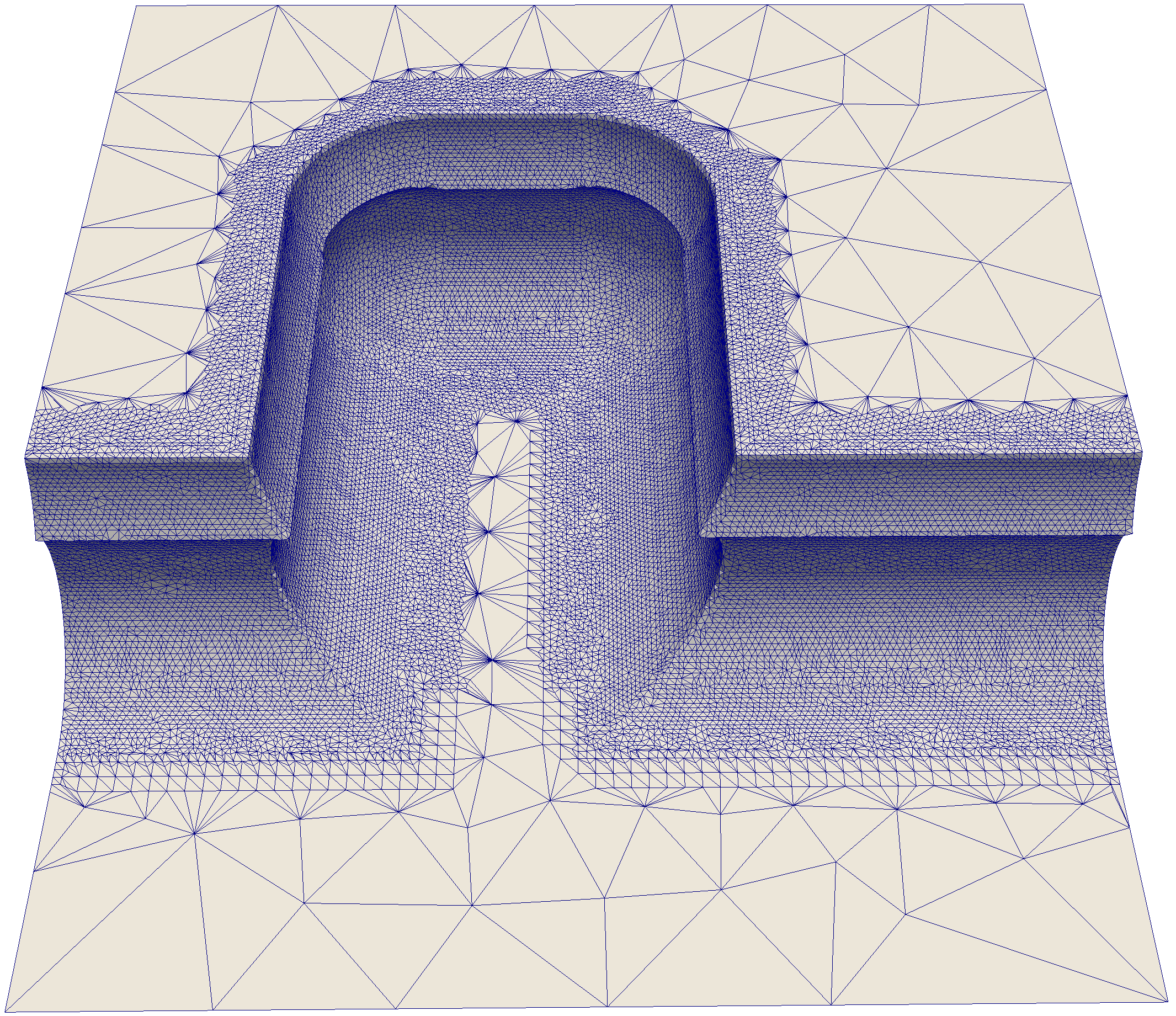
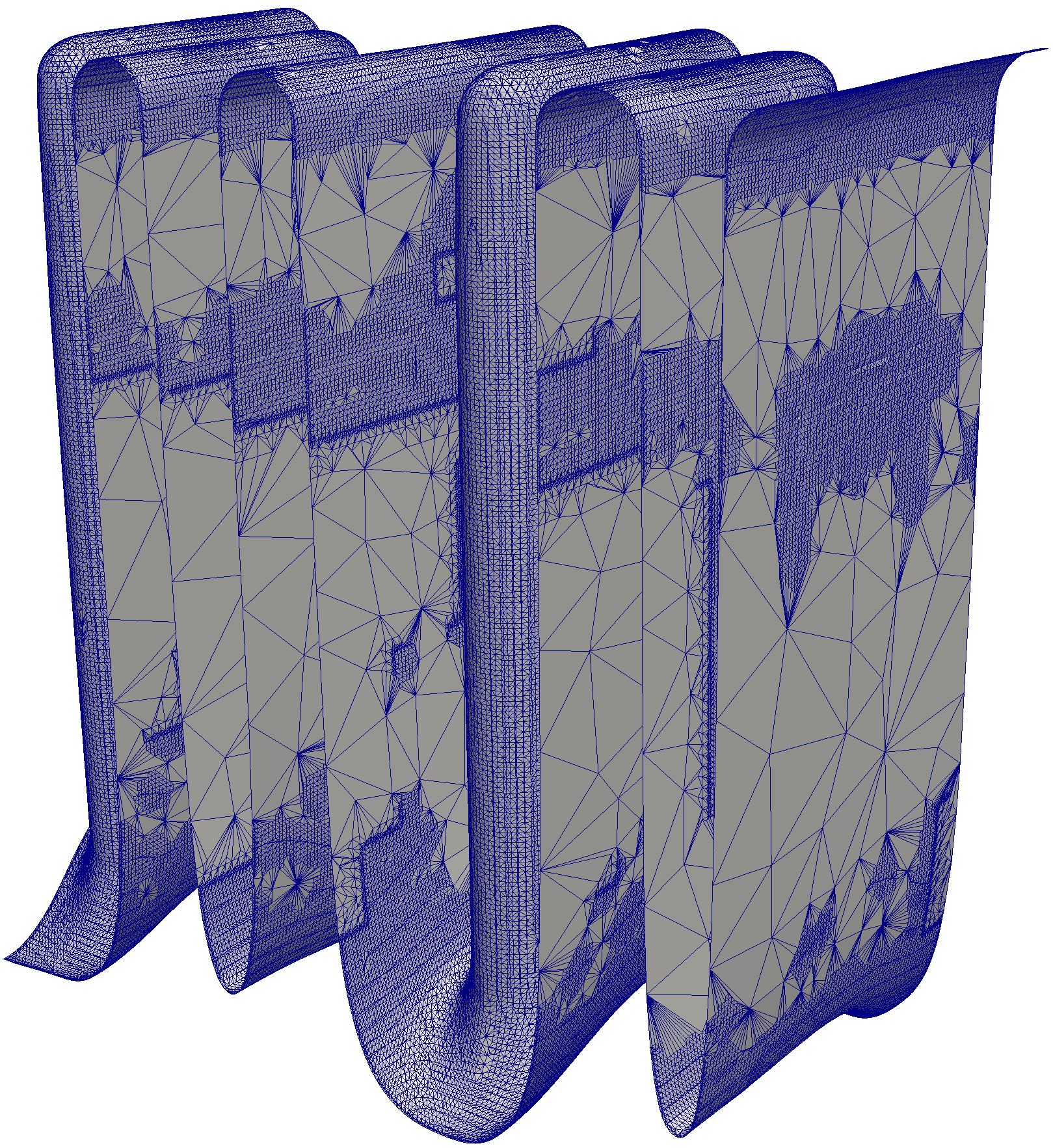
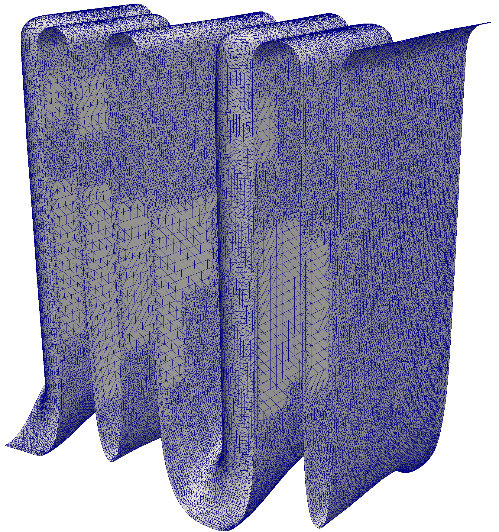
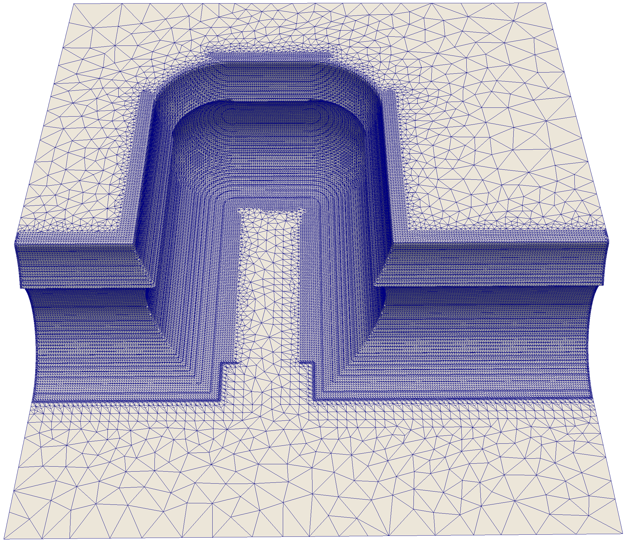
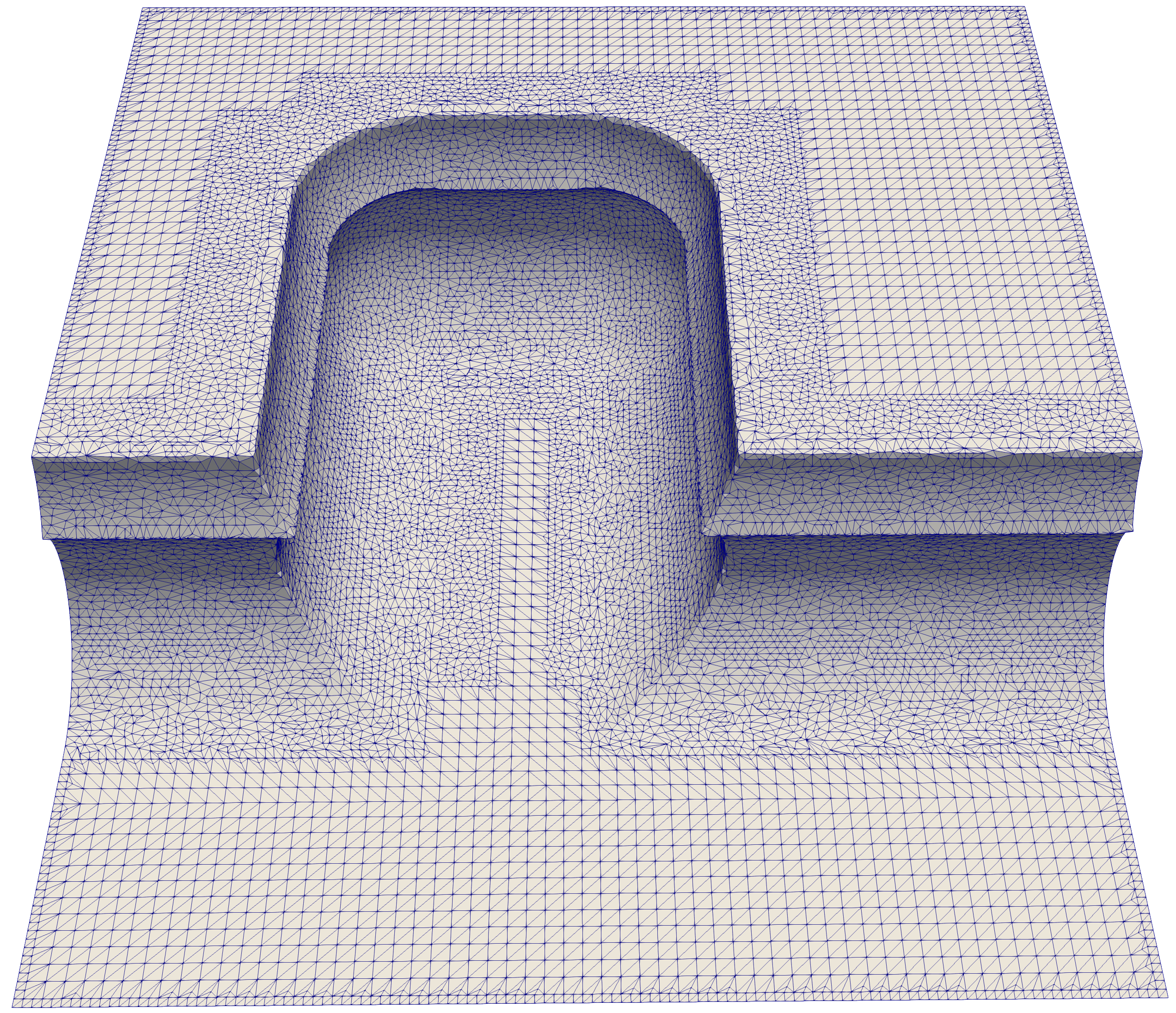
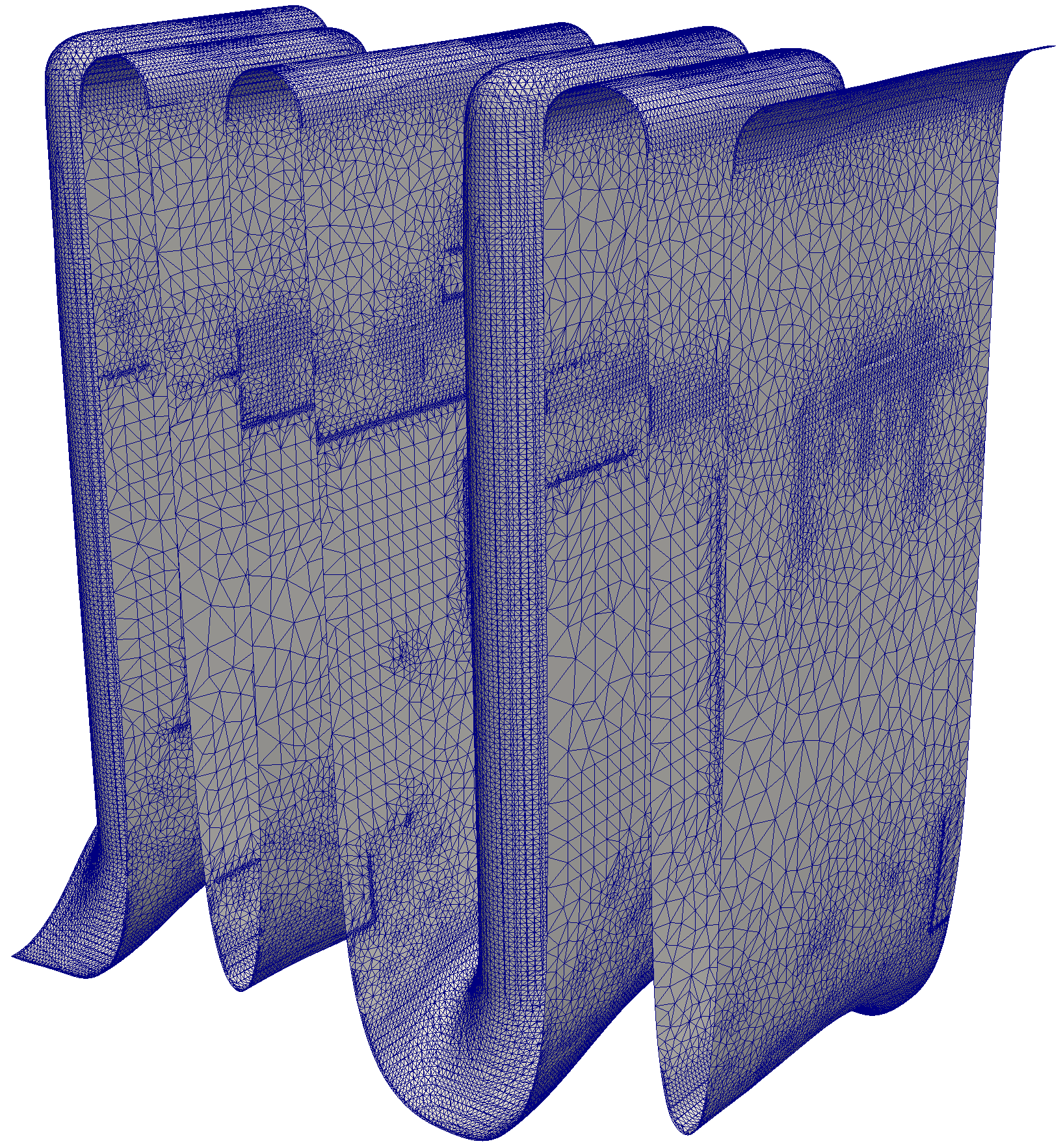
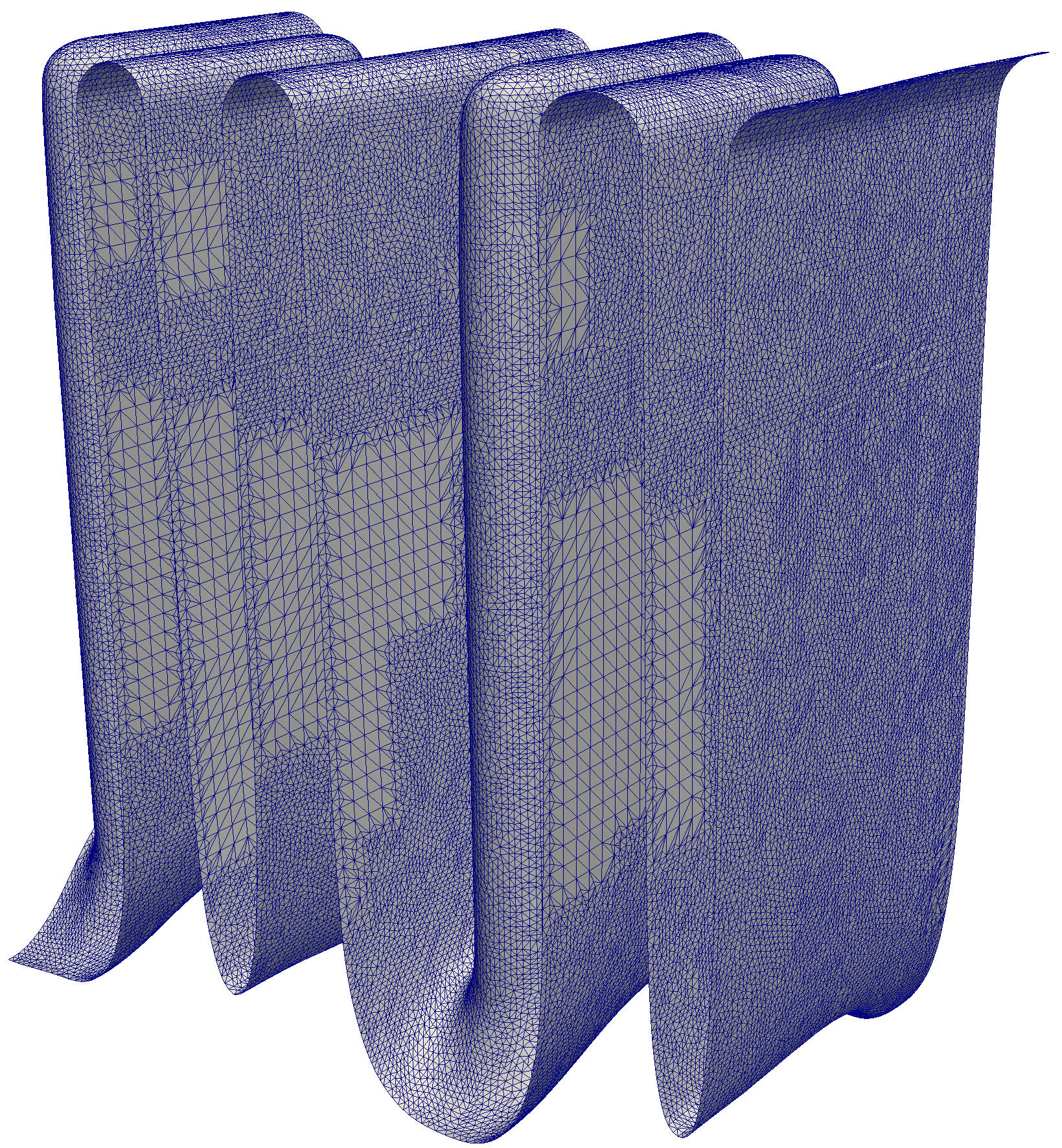
Figure 8.1 shows two example geometries extracted from a process TCAD simulation utilizing hierarchical grids and a marching cubes algorithm.


These figures illustrate that the marching cubes algorithm generates a considerable amount of triangles in flat regions of the geometry, which stem from the discretization of the level-set function on the grid. Obviously, improving the performance of any algorithm operating on such dense surface meshes, e.g., ray tracing, the number of mesh elements must be drastically reduced whilst preserving the features of the geometry.
Reducing the number of elements of a surface mesh is widely studied in computer graphics and is often referred to as surface mesh simplification. Several algorithms exist that simplify surface meshes with respect to a given metric [153, 154, 155, 156]. On the one hand, these algorithms operate in such a way that all triangles have approximately the same size [153, 154], thus, homogeneously simplifying the surface mesh. On the other hand, these algorithms use computationally expensive metrics during the simplification process [155, 156]. Both of these strategies have drawbacks when applied during a process TCAD simulation. A homogenous simplification of the entire surface may lead to the degradation of topographical features when a significant amount of surface elements is removed. Although a simplified surface mesh using an algorithm with an expensive metric may result in a suitable representation of the topography, such an approach is prohibitive since the surface flux calculation has to be performed in every time step. These constraints lead to the following consideration: To efficiently simplify a surface mesh extracted with the marching cubes algorithm, a computationally performant simplification strategy is required that is aware of the previously indicated feature of the geometry. Therefore, this chapter introduces a combination of the feature detection algorithm introduced in Section 5.1.2 with a surface mesh simplification algorithm using a computationally efficient metric (e.g., the Lindstrom-Turk algorithm [153]) to realize a so-called region simplification algorithm. The developed algorithm is evaluated using problem cases originating from process TCAD simulations, underlining practical application.
Section 8.1 introduces the edge collapse and Lindstrom-Turk algorithm, which are the fundamental algorithms used for mesh simplification in this work. Next, the developed region simplification algorithm is introduced (Section 8.2), which simplifies features of the geometry to a lower degree than non-features, allowing for a significantly improved balance between number of mesh elements and feature preservation. In the last section of this chapter (Section 8.3) the performance of the region simplification algorithm is evaluated. The geometric error introduced by the simplification is analyzed by calculating the Hausdorff-distance between the original and simplified surface meshes. Furthermore, the region simplification and the ray tracing run-times are evaluated.
Own Contributions
8.1 Surface Mesh Simplification
This section introduces the underlying, key algorithms used for the developed region simplification algorithm presented in Section 8.2. First, the edge collapse algorithm is presented, which provides the basic mechanism to remove elements from the mesh. Next, the Lindstrom-Turk algorithm is discussed, which provides the basic metrics to decide which mesh elements should be removed.
8.1.1 Edge Collapse Algorithm
As previously mentioned, the utilized algorithm for surface mesh simplification is the edge collapse algorithm [159]. This algorithm requires three functions: First, a weight function that determines which edge should be removed. Second, a placement function that determines a point in space where a new vertex is placed after an edge is removed from the surface mesh. Third, a termination function which stops the simplification process.
The algorithm starts by calculating the weight of all edges (see Section 8.1.2) in the surface mesh and storing them in a minimum heap \(\mathcal {h}\). Afterwards, the edge with the lowest weight is chosen; this edge is removed from the surface mesh and replaced by a vertex. For the new vertex, a position is calculated (see Section 8.1.2), and all edges that were previously connected to the vertices of the removed edge are connected to the newly created vertex. Figure 8.2 shows an illustration of this process. Next, the weights of the affected edges are recalculated and put into the heap \(\mathcal {h}\). This process is repeated until the termination function ends the simplification process. Each collapsed edge removes one vertex, two triangles, and three edges from the surface mesh. In this work, the following two termination criteria are used:
-
• If the edge length of the to be removed edge is larger than a user supplied edge length (\(l_{\max }\)).
-
• If no edges have been removed in the previous simplification step.

8.1.2 Lindstrom-Turk Algorithm
The method used to calculate the weights of the edges and the position of the newly placed vertices is provided by the Lindstrom-Turk algorithm [153]. This algorithm is based on four constraints that aim to minimize the change in the volume characterized by the surface mesh. These four constraints are boundary preservation, volume preservation, volume optimization, and triangle shape optimization. Depending on the examined edge, three of the four constraints are chosen. Each constraint can then be interpreted as a plane in \(\mathbb {R}^3\), which is linearly independent of the planes of the other constraints. The intersection point of these three planes describes the optimal position (i.e., the minimal change in volume after the edge is removed) of the to be placed vertex, and the weight of the edge is determined by the weighted (a user supplied parameter) sum of all optimization parameters.
The Lindstrom-Turk algorithm allows for an efficient calculation of the weights of the edges as well as the position of the new vertex. Furthermore, the Lindstrom-Turk algorithm takes the quality of the newly created triangle into consideration (i.e., aiming to create equilateral triangles).
8.2 Region Simplification Algorithm
The region simplification algorithms start by analyzing the features of the surface mesh, which are used to split the surface mesh into two disjunct so-called feature and transition regions, as will be discussed in detail below. These regions can then be simplified using different strategies, allowing for a higher resolution at features of the geometry. In this work, the Lindstrom-Turk algorithm with different parameter sets is used to guide the simplification process in both regions of the surface mesh, however, the region simplification algorithm is not limited to the Lindstrom-Turk algorithm. Thus, other simplification methods can be used to simplify the transition and feature region respectively.
This section starts by discussing the feature detection strategy. Next, it is described how the detected features are used to split the mesh into regions. Finally, the simplification of the different regions and a strategy to create a smooth transition from smaller to bigger mesh elements is discussed.
8.2.1 Feature Detection
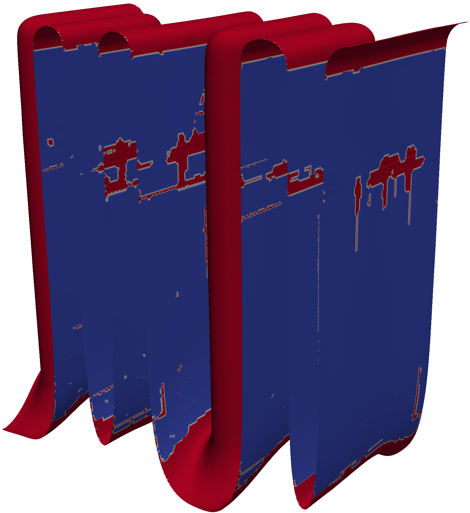
The simplification algorithm starts by performing a feature detection on the entire surface mesh. This is achieved by using the feature detection algorithm from Section 5.1.2 and applying it to the vertices of the surface mesh. Furthermore, the mean (\(H\)) and Gaussian curvature (\(K\)) for the vertices are calculated with the curvature calculation methods presented in Section 3.3. The feature detection algorithm, with a feature detection parameter of \(C=0.5\), is used to classify each vertex in the surface mesh as either a flat or a feature vertex. A vertex is considered to be a feature vertex if it is detected as a feature and flat otherwise. An illustration of the detected features on the two surface meshes introduced in Figure 8.1 is shown in Figure 8.3.

8.2.2 Mesh Partitioning and Extension of Regions
As previously mentioned, the detected features are used to partition the surface mesh into regions, the feature regions (i.e., feature vertices) and the transition regions (i.e., flat vertices). The partitioning of the mesh allows the surface mesh simplification algorithm to simplify the transition region to a greater extent. Thus, removing more mesh elements from flat parts of the geometry while maintaining a higher resolution at features of the surface mesh. However, the straightforward approach of only simplifying triangles in the transition region up to a fixed edge length produces a significant number of low quality triangles (see Section 2.2), as can be seen in Figure 8.4.
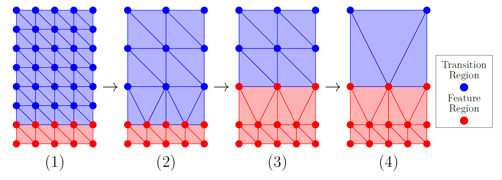
Therefore, the region simplification utilizes a mesh grading that linearly increases the edge length of the triangles the further they reach into the transition region, to minimize the number of low quality triangles. This is achieved in the following way: After the feature region and the transition region are identified, the iterative simplification algorithm starts by simplifying the entire surface mesh, including the feature region, with a minimum edge length of \(l_0\). In the case that the feature region should not be simplified, \(l_0\) is set to \(0\). The subsequent simplification step starts at the border between the transition and the feature region. The transition region is simplified until a minimal edge length of \(l_{1} = l_0 + sl\), where \(sl\) denotes a user specified step length, is reached. Next, the feature region is extended into the transition region (i.e., moved) by adding all vertices that are adjacent (e.g., connected by an edge) to the feature region. The contracted transition region is again simplified until a minimal edge length of \(l_{i+1} = l_i + sl\) with \(i \in \{0,1,\dots ,n \in \mathbb {N}\}\) is reached. These last two steps continue until one of the two termination conditions introduced in Section 8.1.1 is fulfilled, thus, terminating the simplification process. Figure 8.5 illustrates the above discussed extension and, subsequent, simplification of the regions.
Furthermore, Figure 8.6 depicts a flow chart of the simplification process.

To avoid the generation of too large triangles in this iterative scheme, the previously mentioned parameter \(l_{\max }\) can be chosen accordingly. This terminates the simplification process when the minimal edge length in the transition region \(l_i\) has reached an edge length equal or larger than \(l_{\max }\). In a surface mesh extracted from a level-set function, the parameter \(l_0\) can be chosen in concordance with the smallest sub-grid resolution \(\Delta x\). For other surface meshes, the parameter \(l_0\) can be chosen by averaging the length of all edges in the feature region. Furthermore, empirically it has been observed that the step length \(sl\) should not be chosen bigger than \(l_0\): Although the amount of mesh elements would be reduced by choosing a larger parameter, the triangle quality of the surface mesh suffers.
8.3 Comparison and Evaluation
The region simplification algorithm is evaluated with respect to three metrics:
-
• The distance between the original and simplified surface mesh (i.e., the error introduced by the simplification).
-
• The run-time of the simplification process.
-
• The run-time of surface flux calculations using Monte Carlo ray tracing.
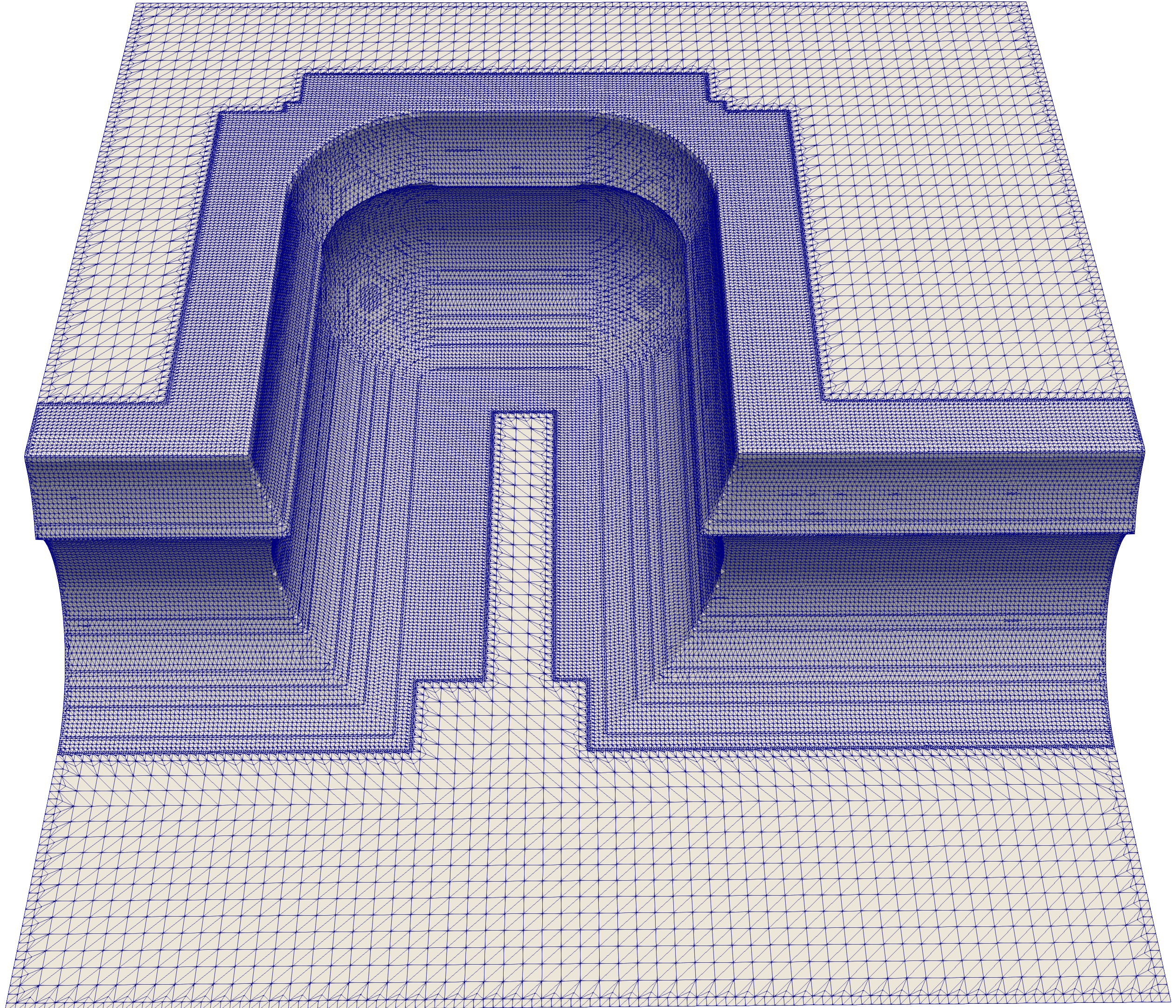
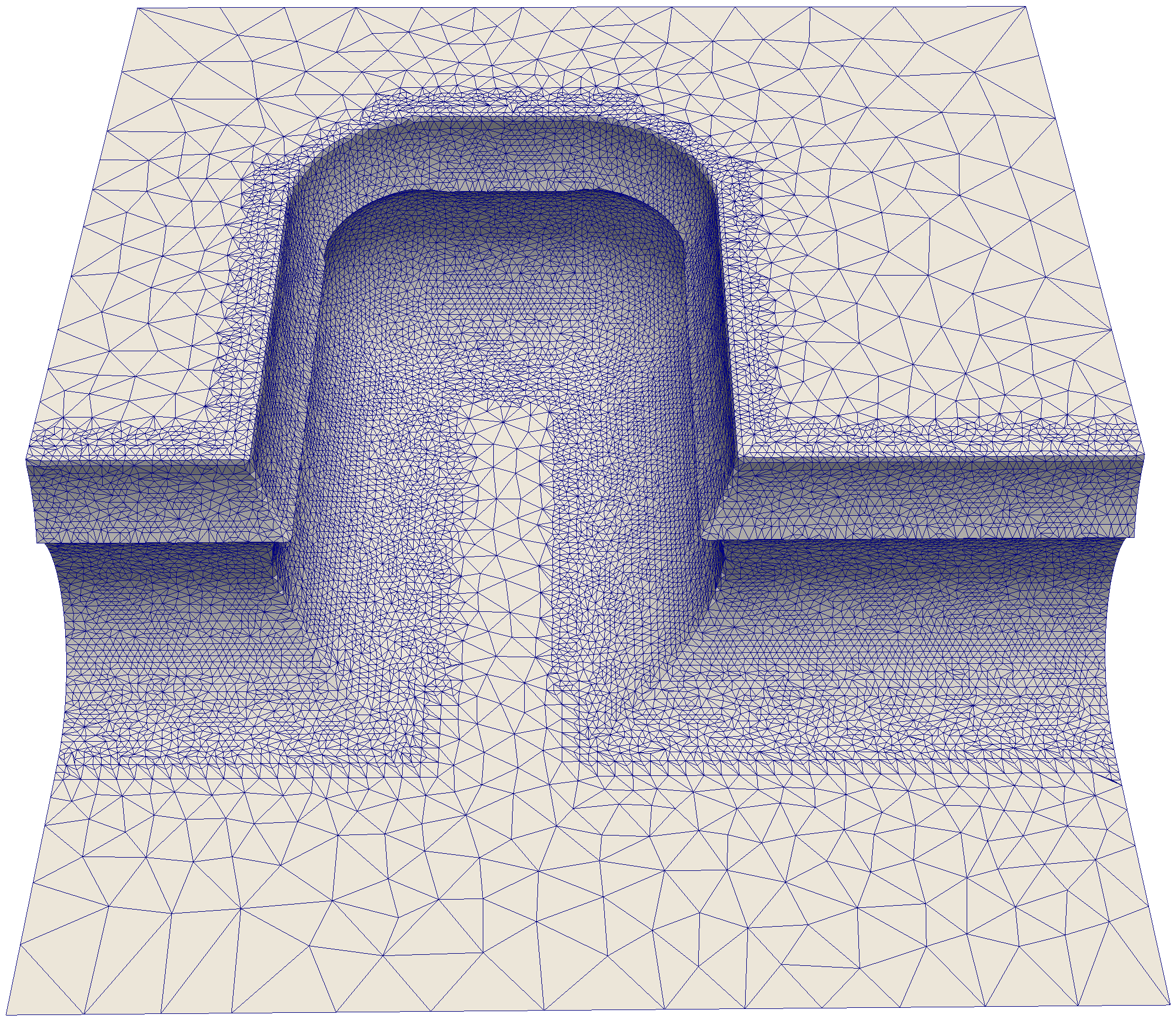
To that end, the two example meshes (see Figure 8.1) are simplified using the region simplification algorithm and the Lindstrom-Turk algorithm. Each of the example meshes is simplified using eight different parameter sets, which reduced the number of vertices in the mesh by \(20\) to \(90 \%\). An exemplary, comparative result is shown in Figure 8.7.

This comparison illustrates that the region simplification algorithm primarily removes triangles in the flat region and keeps a higher resolution at the features of the geometry. The surface meshes have been simplified using ViennaMesh and CGAL and were executed on the benchmark platform Workstation 1 (see Section 4.6.3).
8.3.1 Distance to Original Geometry
The simplification process introduces minor errors in the discretization of the surface. Although the Lindstrom-Turk algorithm tries to minimize this error, it is unavoidable since each edge collapse removes information about the surface. Thus, a metric is required that is able to capture the introduced error and allows to compare the two algorithms. A commonly used metric that calculates the distance between two sets (e.g., surface meshes) is the Hausdorff distance [160]. The Hausdorff distance is defined as follows [161]:
8.3.1 Definition (Hausdorff Distance) Let \(X, Y \subset \mathbb {R}^3\) be two sets. Then the Hausdorff distance is defined as:
\(\seteqnumber{0}{8.}{0}\)\begin{align*} d_{H}(X, Y) = \text {max} (d_{H'}(X, Y), d_{H'}(Y, X)). \end{align*}
\(d_{H'}(X, Y)\) stands for the one-sided Hausdorff distance:
8.3.2 Definition (One-Sided Hausdorff Distance) Let \(X, Y \subset \mathbb {R}^3\) be two sets. Then the one-sided Hausdorff distance is defined as follows:
\(\seteqnumber{0}{8.}{0}\)\begin{align*} d_{H'}(X, Y) := \max _{\mathbf {p} \in X} (\min _{\mathbf {q} \in Y} (\| \mathbf {p} - \mathbf {q} \|)). \end{align*}
In the case of surface meshes, the Hausdorff distance is measured from the vertices of one surface mesh to the closest triangle intersection of the other surface mesh [161]. The error introduced by the simplification process is determined by calculating the Hausdorff distance from the original geometry (e.g., the not simplified surface mesh) to the simplified surface mesh.
Figure 8.8 and Figure 8.9 show the simplified Surface 1 and the Hausdorff distances to the original geometry.


The Hausdorff distances reported in Figure 8.8c show that there is no geometric error introduced into the simplified geometry, since the region simplification algorithm does not simplify the feature region (i.e., \(l_0 = 0\)). Furthermore, this indicates that the feature detection is able to detect all features of the surface mesh correctly and thus only simplifies triangles in flat parts of the surface mesh, which does not alter the geometry represented by the surface mesh. On the other hand, when the feature region is simplified, to achieve an overall higher degree of simplification, geometric errors are introduced into the simplified surface mesh, as can be seen in Figure 8.9c. The smaller geometric error is a consequence of the feature region being simplified to a lesser degree and more elements are removed from the flat region when using the region simplification algorithm compared to the Lindstrom-Turk algorithm. Nevertheless, the surface mesh simplified with the region simplification algorithm has a smaller error than the one simplified with the Lindstrom-Turk algorithm.
Figure 8.10 and Figure 8.11 again show the Hausdorff distances to the original geometry and the simplified surface mesh of Surface 2.


First, it has to be mentioned that the average Hausdorff distance of Surface 2 is one order of magnitude smaller than that of Surface 1. The reason for that difference is the base grid resolution of the underlining simulation from which the two meshes where extracted. In Figure 8.10c, a small error in the Hausdorff distance can be seen, even though the feature region is not simplified. This error occurs since Surface 2 has finer features than Surface 1, which are not captured by the feature detection algorithm. However, in general, a small error in the feature detection is to be expected since a feature detection parameter has to be used (see Section 5.1), which is going to miss features smaller than the feature detection parameter. Additionally, the surface mesh simplified with region simplification has a far smaller error than the mesh simplified with the Lindstrom-Turk algorithm, since it removes more mesh elements from the transition region than from the feature region, which is further confirmed in Figure 8.11c for the case of simplifying the feature region.
On average region simplification has a \(20\) - \(40\) % lower Hausdorff distance to the original geometry than using the Lindstrom-Turk algorithm. Next, the simplification run-times of the two simplification algorithms are investigated to study the computational effort of both simplification algorithms.
8.3.2 Simplification Run-Time
The simplification run-times of the example meshes using the different parameters are reported in Figure 8.12.


As expected, it is shown that region simplification introduces an overhead into the simplification process compared to the Lindstrom-Turk algorithm. The main reason is the feature detection used to split the surface mesh into regions. Compared to the Lindstrom-Turk algorithm, region simplification has, on average, a 17 % longer simplification time. However, when considering entire process TCAD workflows (see Section 4.5), the additional time spent on improved surface mesh simplification easily pays of with costly subsequent process simulation steps, such as ray tracing for flux calculations, as significantly less triangles have to be processed.
8.3.3 Flux Calculation and Monte Carlo Ray Tracing Run-Time
The run-times of flux calculations using Monte Carlo ray tracing based on the simplified example meshes (see Figure 8.1) are shown in Figure 8.13.


It is shown that the speedup of the ray tracing also depends on the underlying geometry. For geometries that represent deep trenches (i.e., Surface 2), the speedup achieved by the surface mesh simplification is more dependent on the size of the triangles than for geometries with smaller horizontal variation(i.e., Surface 1). These differences are explained by the difference in the bounding volume hierarchy (i.e., the data structure used for ray tracing), which can be traversed faster in a deep trench with bigger elements. When tracing Surface 1, the simplified surface meshes improve the run-times of the flux calculation. Furthermore, both simplification methods perform similarly to each other. The run-times of ray tracing performed on Surface 2 are also improved by the surface mesh simplification. Additionally, the surface meshes simplified with the region simplification algorithm outperform the meshes simplified with the Lindstrom-Turk algorithm. The biggest ray tracing performance differences between the two algorithms is about 12 % at the simplification levels between 52 and 67 %.
Comparing the run-times for the surface mesh simplification (see Figure 8.12) and the ray tracing (see Figure 8.13) shows that the speedup achieved for the ray tracing on the simplified surface meshes is bigger than the cost of simplifying the surface mesh, confirming the previously stated justification in Section 8.3.2.
8.4 Summary
A new surface mesh simplification algorithm has been presented. The algorithm uses the features of a surface mesh to divide it into disjunct regions that are simplified with different parameters. The algorithm is well suited for surface meshes originating from process TCAD simulations used for surface flux calculations. The surface mesh simplification algorithm has been evaluated by investigating the distance to the original geometry, the run-times of the surface mesh simplification, and a subsequent flux calculation step using Monte Carlo ray tracing. Surface meshes simplified with the proposed surface mesh simplification algorithm have an improved geometric distance to the original surface mesh compared to a surface mesh simplified with the reference algorithm. The average Hausdorff distance of the investigated geometries is improved by \(20\) - \(40\) %. On average, the ray tracing performance on the simplified surface meshes is improved by \(15\) %. Additionally, geometries from process TCAD simulations with deep trenches, simplified with the region simplification algorithm, perform much better in ray tracing. The time spent on simplification is, on average, \(17\) % slower when using region simplification compared to the reference algorithm. Therefore, when considering the entire process of flux calculation, the acceleration of the ray tracing due to the simplified surface exceeds the time spent on surface mesh simplification, underlying the importance of surface mesh simplification in relevant process TCAD workflows.