

Computation of Torques
in Magnetic Tunnel Junctions
Chapter 3 Micromagnetics Modeling
Simulation tools are a powerful help in the design of modern STT-MRAM devices. Micromagnetics modeling allows to have a description of the evolution in time of the magnetization, described as a continuous quantity. The
following chapter gives a brief overview of the magnetization dynamics’ modeling via the Landau-Lifschitz Gilbert equation. The contents are mostly based on references [17],
[83], and [84].
3.1 Landau Lifshitz Gilbert Equation
The explanation of ferromagnetism on the basis of exchange interactions, developed by Heisenberg and Dirac in 1928, created the possibility of developing a mesoscopic theory of magnetism which combined Maxwell’s equations and quantum theory. The first description of time dependent motion of magnetic moments presenting no exchange coupling and without energy dissipation, thus in the absence of damping, was reported by Bloch in 1932 [85]. Landau and Lifshitz proposed a continuous equation for the description of the damped motion of the magnetization in a ferromagnet in 1935 [86]. Such a description was strictly valid only for small damping. A formulation which could be employed to describe strong damping in thin films was then developed by Gilbert in 1955 [87]. Following the work by Gilbert, a derivation of the equation of motion for the magnetization dynamics from considerations of the magnetic moment of electrons is hereby presented.
The magnetic moment represents the strength and orientation of the magnetic dipole of an object. It can be defined as the vector describing the relation of an external magnetic field to the torque it exerts on the object generating the moment itself. Such relationship is given by
\(\seteqnumber{0}{3.}{0}\)\begin{equation} \bm {\tau } = \bm {\mu } \times \vb {B} \, , \label {eq:mag_moment} \end{equation}
where \(\bm {\tau }\) is the torque, \(\bm {\mu }\) is the magnetic moment, and \(\vb {B}\) is the magnetic induction. Given the presence of a torque acting on an object, the equation describing its rotational motion is
\(\seteqnumber{0}{3.}{1}\)\begin{equation} \pdv {\vb {L}}{t} = \bm {\tau } \, , \label {eq:rot_motion} \end{equation}
where \(\mathbf {L}\) is the angular momentum of the particle. The relation of the magnetic moment of an electron and its angular momentum is described by
\(\seteqnumber{0}{3.}{2}\)\begin{equation} \boldsymbol {\mu } = \gamma \mathbf {L} \, , \label {eq:mag_ang_relation} \end{equation}
where \(\gamma \) is the gyromagnetic ratio of the electron. By putting equations (3.1) and (3.3) into (3.2), one obtains the following equation of motion:
\(\seteqnumber{0}{3.}{3}\)\begin{equation} \pdv {\boldsymbol {\mu }}{t} = \gamma \boldsymbol {\mu } \times \mathbf {B} \label {eq:mag_mom_motion} \end{equation}
Equation (3.4) is satisfied by a single magnetic moment. In micromagnetism, the magnetization is considered a continuous vector quantity, which takes the place of the single magnetic moment in the equation of motion previously described. Moreover, in the case of constant temperature and uniform density of spins, which is often considered for micromagnetic simulations, the continuous magnetization \(\vb {M}\) has a constant value and can thus be written in terms of a unit vector \(\vb {m}\) as
\(\seteqnumber{0}{3.}{4}\)\begin{equation} \label {eq:magnetization} \vb {M} = M_\text {S}\,\vb {m},\qq {with}|\vb {m}|=1 \, , \end{equation}
where the saturation magnetization \(M_\text {S}\) is a material parameter. The quantity \(\vb {m}\) will be referred to as magnetization throughout this thesis. In order to derive a general equation of motion, the magnetic induction is replaced with an effective field \(\vb {H}_\text {eff}\), which describes not only the effects of an externally induced magnetic field, but also of contributions intrinsic to the ferromagnet, as will be clarified in Section 3.2. By taking the rescaled value of the gyromagnetic ratio \(\gamma _0=-\gamma \,\mu _0\), the equation of motion for the magnetization takes the following form:
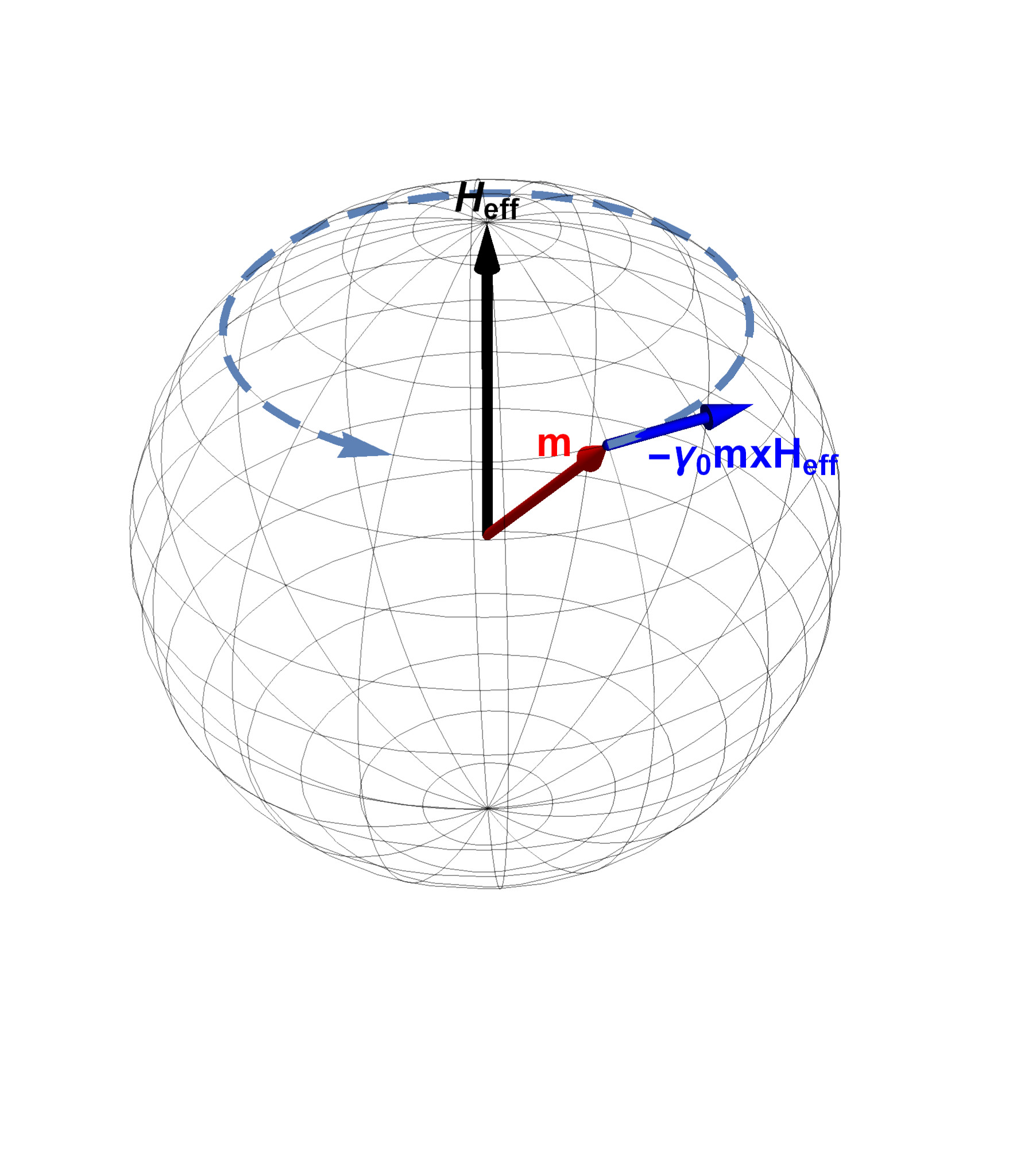
\(\seteqnumber{0}{3.}{5}\)\begin{equation} \pdv {\vb {m}}{t} = -\gamma _0 \, \vb {m} \times \vb {H}_\text {eff} \label {eq:mag_motion} \end{equation}
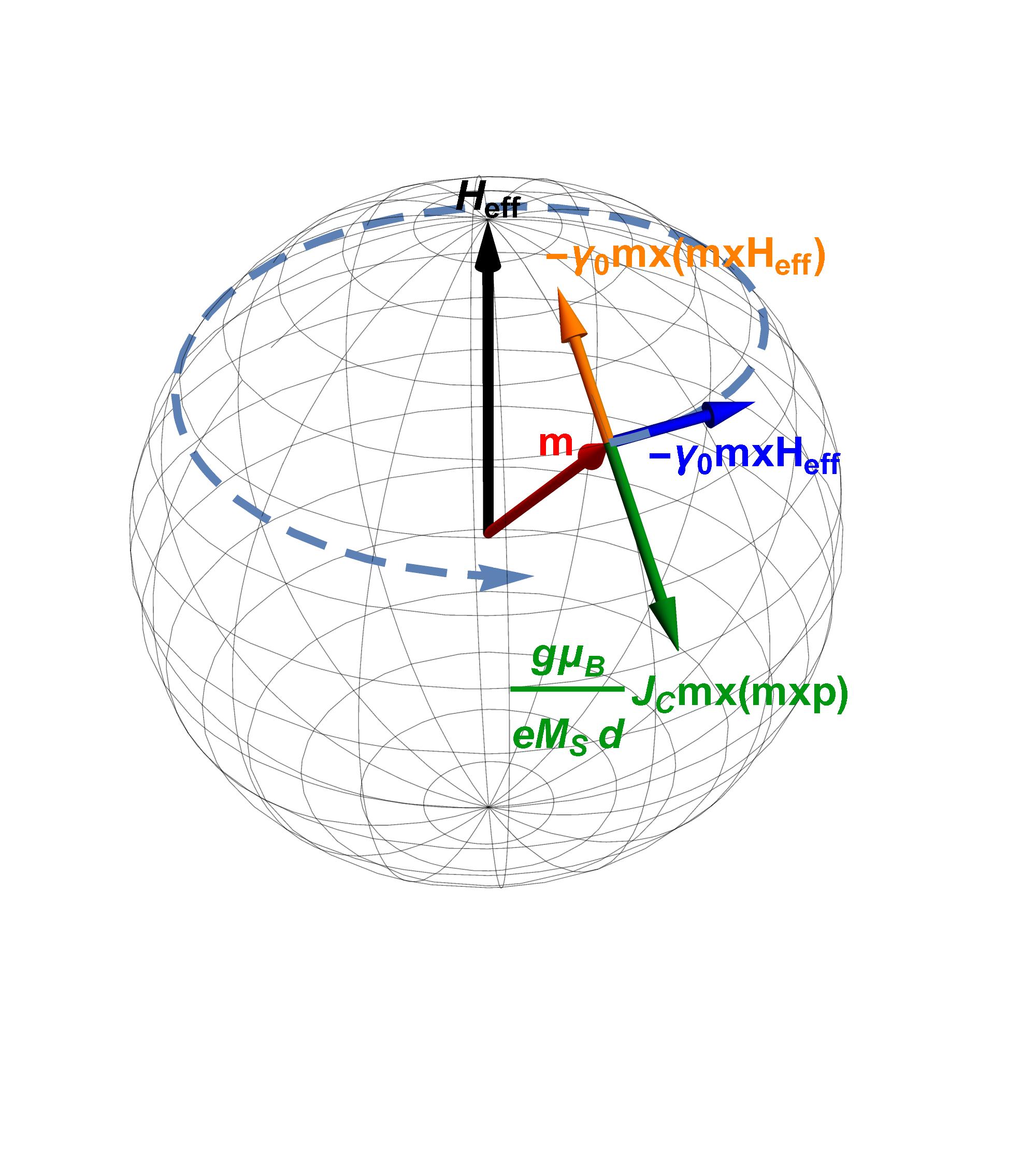
The equation derived until now describes a precessional motion of the magnetization around the magnetic field, see Fig. 3.1. From experiments, however, the magnetization dynamics is dissipative. The effect of an energy loss mechanism can be introduced in the equation in a phenomenological way, taking into consideration two main aspects: the damping process should lead the magnetization relaxing parallel to the effective field, as to minimize the energy, and it should not affect the magnetization magnitude (see Fig. 3.2(a)). This was first done in 1935 by L. D. Landau and E. M. Lifshitz, resulting in the so called Landau-Lifshitz equation [86]:
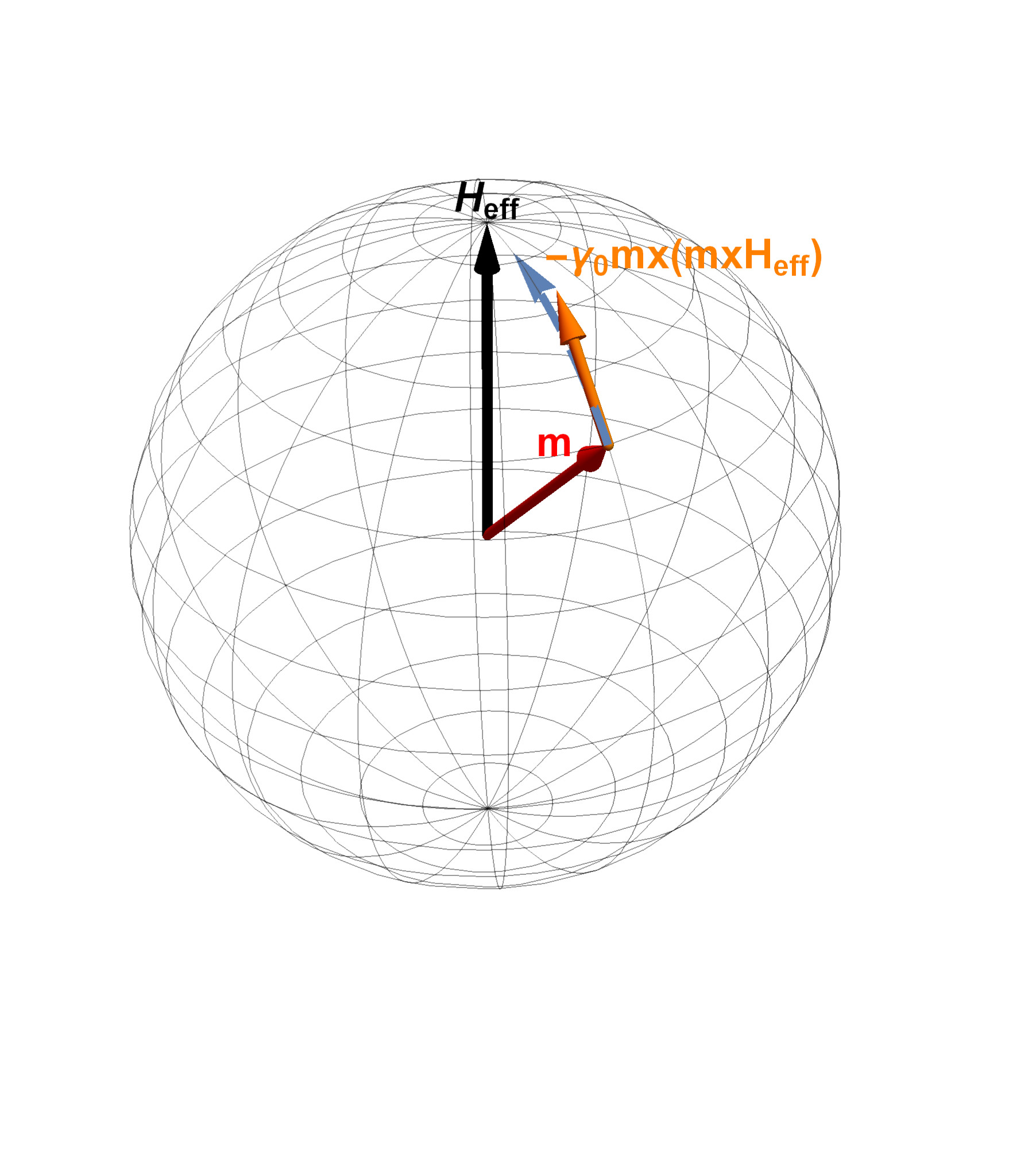
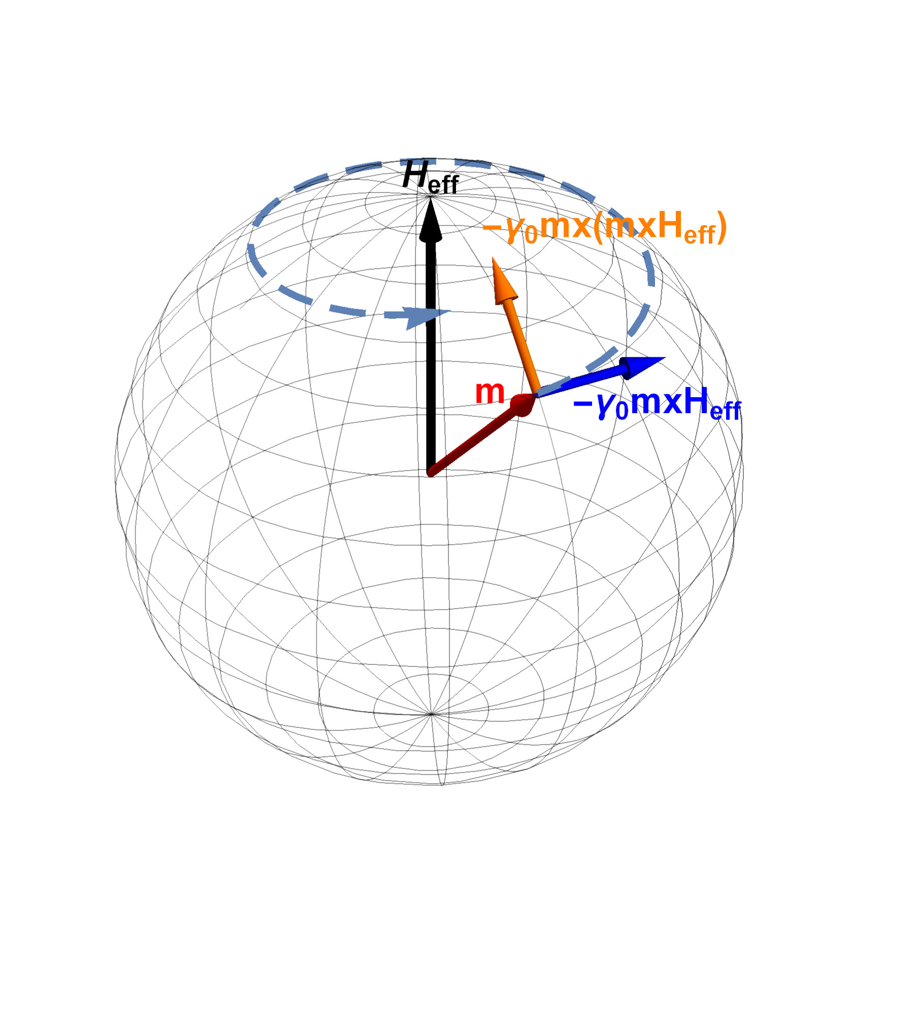
\begin{equation} \pdv {\vb {m}}{t} = -\gamma _0 \, \vb {m} \times \vb {H}_\text {eff} -\gamma _0 \lambda \, \vb {m} \times \left ( \vb {m} \times \vb {H}_\text {eff} \right ) \label {eq:ll} \end{equation}
\(\lambda \) > 0 is a dimensionless phenomenological damping parameter, which can be determined experimentally and is material dependent. The proposed equation describes a magnetization rotating around the effective magnetic field and being slowly quenched towards it (see Fig. 3.2(b)). The speed of the damping process is determined by the magnitude of \(\lambda \). In order to deal with situations in which a strong damping is present, in 1955 T. L. Gilbert proposed a modified equation with a different form of the damping term, to be taken directly proportional to the time derivative of the magnetization [88]. The modified equation reads as
\(\seteqnumber{0}{3.}{7}\)\begin{equation} \pdv {\vb {m}}{t} = -\gamma _0 \, \vb {m} \times \left ( \vb {H}_\text {eff} - \zeta \, \pdv {\vb {m}}{t} \right ) \, , \label {eq:gilbert_1} \end{equation}
where \(\zeta \) is a viscosity parameter. By separating the two vector products, the equation takes the form
\(\seteqnumber{0}{3.}{8}\)\begin{equation} \pdv {\vb {m}}{t} = -\gamma _0 \, \vb {m} \times \vb {H}_\text {eff} + \alpha \, \vb {m} \times \pdv {\vb {m}}{t} \, , \label {eq:gilbert} \end{equation}
where \(\alpha =\gamma _0 \zeta \) is a dimensionless parameter referred to as Gilbert damping constant. In this formulation, the equation is known as Gilbert equation. It can be noted that equations (3.7) and (3.9) are equivalent, up to the rescaling of the constants. By cross-multiplying both sides of equation (3.7) by \(\vb {m}\), by employing the triple product expansion formula and by taking into consideration the constraint \(|\vb {m}|=1\), it can be rewritten as
\(\seteqnumber{0}{3.}{9}\)\begin{equation} \pdv {\vb {m}}{t} = -\gamma _0 \, (1+\lambda ^2) \, \vb {m} \times \vb {H}_\text {eff} + \lambda \, \vb {m} \times \pdv {\vb {m}}{t} \, . \label {eq:ll_mod} \end{equation}
Using the same procedure on equation (3.9), it can be expressed as
\(\seteqnumber{0}{3.}{10}\)\begin{equation} \pdv {\vb {m}}{t} = -\frac {\gamma _0}{1+\alpha ^2} \, \vb {m} \times \vb {H}_\text {eff} -\frac {\gamma _0\alpha }{1+\alpha ^2} \vb {m} \times \left ( \vb {m} \times \vb {H}_\text {eff} \right ) \, . \label {eq:gilbert_mod} \end{equation}
Equation (3.11) is commonly referred to as the Landau–Lifshitz–Gilbert (LLG) equation. Throughout the thesis, the Gilbert form of the damping will be employed.
3.2 Effective Field
In order to derive an expression for the various contributions to the effective field the magnetic Gibbs free energy of a ferromagnetic body must first be defined. Such quantity, indicated as \(\mathcal {E}\), includes various contributions, such as the exchange energy, the anisotropy energy, the energy from an applied external field, and the magnetostatic energy. Such contributions will be described more in detail in the following sections. Once an expression for the Gibbs energy is known, a stable configuration of the magnetization is one that minimizes it, leading to the minimization problem
\(\seteqnumber{0}{3.}{11}\)\begin{equation} \min _{|\mathbf {m}|=1} \mathcal {E}(\mathbf {m}) \, . \label {eq:min_energy} \end{equation}
A stable magnetization configuration constitutes a balancing point between the energy contributions. The effective field acting on the magnetization in the LLG equation stems directly from this minimization problem, and is defined as the functional derivative of the magnetic Gibbs free energy with respect to the magnetization [89]:
\(\seteqnumber{0}{3.}{12}\)\begin{equation} \mu _0 M_\text {S} \, \vb {H}_\text {eff} = -\fdv {\mathcal {E}(\vb {m})}{\vb {m}} \label {eq:heff} \end{equation}
In fact, from the Euler-Lagrange equations associated to (3.12), it stems that any solution to it is also a solution to the boundary value problem
\(\seteqnumber{1}{3.14}{0}\)\begin{align} \vb {m} \times \vb {H}_\text {eff} & = 0 \, ,\\ \fdv {\mathcal {E}(\vb {m})}{\grad {m_i}} \cdot \vb {n} & = 0,\qq {for} 1 \leq i \leq 3 \, . \label {eq:bdr_cond} \end{align} \(\vb {n}\) is the unit vector normal to the external boundary of the ferromagnetic domain under investigation. It can be noted that a configuration minimizing the energy requires the magnetization vector to be parallel to the local effective field. It is then clear that the process described by the LLG equation is a relaxation towards a state with minimal energy. The effective field contributions considered throughout this thesis are the following:
\(\seteqnumber{0}{3.}{14}\)\begin{equation} \vb {H}_\text {eff} = \vb {H}_\text {exc} + \vb {H}_\text {ani} + \vb {H}_\text {ext} + \vb {H}_\text {demag} + \vb {H}_\text {th} \label {eq:heff_cont} \end{equation}
\(\vb {H}_\text {exc}\) is the exchange field, \(\vb {H}_\text {ani}\) is the anisotropy field, \(\vb {H}_\text {ext}\) is the external field, \(\vb {H}_\text {demag}\) is the demagnetizing field, also called magnetostatic field, and \(\vb {H}_\text {th}\) is the thermal field. Each contribution will be described more in detail in the following sections.
3.2.1 Exchange Field
In ferromagnetic materials, it is energetically favorable for magnetic moments of neighboring atoms to be parallel to each other, due to the exchange interaction between them. Such interaction is of quantum mechanical origin, and was first predicted by W. K. Heisenberg in 1926. In micromagnetism which takes into consideration a continuous magnetization vector, this interaction is reflected in an energy contribution which penalizes magnetization variations throughout the magnetic domain, and can be expressed as [89]
\(\seteqnumber{0}{3.}{15}\)\begin{equation} \label {eq:eexc} \mathcal {E}_\text {exc}(\vb {m}) = A \, \int _{\omega }\abs {\grad {\vb {m}}}^2 \dd {\vb {x}} \, , \end{equation}
where \(\omega \) refers to the volume of the ferromagnetic domain, and \(A\) is the exchange coefficient, which is a material dependent parameter expressed in units of J/m. Equation (3.16) exactly represents the lowest order phenomenological energy expression that penalizes inhomogeneous magnetization configurations. By employing the relation (3.13), the exchange field contribution to \(\vb {H}_\text {eff}\) can be derived as
\(\seteqnumber{0}{3.}{16}\)\begin{equation} \label {eq:hexc} \vb {H}_\text {exc} = \frac {2A}{\mu _0 M_\text {S}} \laplacian \vb {m} \, . \end{equation}
3.2.2 Anisotropy Field
In the presence of magnetic anisotropy, the magnetic free energy is minimized by the magnetization lying in one or more preferred orientations, referred to as easy axes. One of the main sources of magnetic anisotropy is given by the properties of the crystalline structure of the material, and is referred to as magnetocrystalline anisotropy. The three most important cases of magnetocrystalline anisotropy are the uniaxial, planar and cubic anisotropy. Each of them is characterized by a different contribution to the magnetic free energy, and so to the effective field [89]. Other sources of magnetic anisotropy include interface effects between different materials (interface anisotropy) and the particular shape of the magnetic domain under consideration (shape anisotropy).
Interface anisotropy is particularly important when discussing magnetic layers with the magnetization perpendicular to the main plane of the structure, and is usually taken into account as a uniaxial anisotropy contribution. The contribution of the shape anisotropy is accounted for by the demagnetizing field, which will be described in section 3.2.4. The origin of the magnetocrystalline and interface anisotropy energy contributions lies in the spin-orbit coupling either due to an anisotropic crystal structure or due to lattice deformation at material interfaces, respectively.
Uniaxial Anisotropy
In the case of uniaxial anisotropy, there is only one preferred direction. In this case, the anisotropy energy, which can be taken as the work necessary to rotate the magnetization away from the easy axis, can be written as
\(\seteqnumber{0}{3.}{17}\)\begin{equation} \mathcal {E}_\text {ani}(\vb {m})=K \, \int _\omega \left (1-\vb {a}\vdot \vb {m}\right )^2 \dd {\vb {x}} \, , \label {eq:uni_anis} \end{equation}
where \(K > 0\) is the material anisotropy coefficient and \(\vb {a}\) is the unit vector identifying the easy axis. A visual representation of the energy distribution described by (3.18) is provided in Fig. 3.3. From (3.13), the anisotropy contribution to the effective field in this case is
\(\seteqnumber{0}{3.}{18}\)\begin{equation} \label {eq:hani_uni} \vb {H}_\text {ani}=\frac {2K}{\mu _0 M_\text {S}}\left (\vb {a}\vdot \vb {m}\right ) \vb {a} \, . \end{equation}
As previously mentioned, an uniaxial anisotropy contribution can be employed to take the interfacial anisotropy, and in particular the PMA acting in pMTJs, into account. The anisotropy coefficient takes in this case the form \(K = K_\text {int}/d_\text {FM}\), where \(K_\text {int}\) is the interface anisotropy, in units of J/m\(^2\), and \(d_\text {FM}\) is the thickness of the FM layer under consideration. The relation between \(K\) and the anisotropy field \(H_\text {K}\) entering (2.2) is given by
\(\seteqnumber{1}{3.20}{0}\)\begin{gather} H_\text {K} = \frac {2 K_\text {eff}}{\mu _0 M_\text {S}} \, , \\ K_\text {eff} = K - \delta N \frac {\mu _0 M_\text {S}^2}{2} \label {eq:K_eff} \, . \end{gather} The second term on the right hand side of (3.20b) stems from the shape anisotropy. \(\delta N\) is the difference between the longitudinal and transverse demagnetizing factors in cylindrical layers, taking positive values for thin layers and negative values for elongated layers [22].
Planar Anisotropy
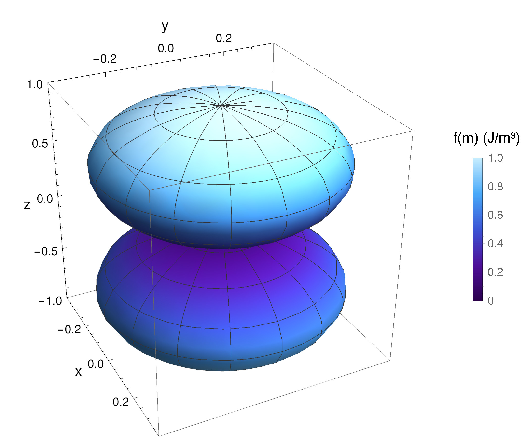
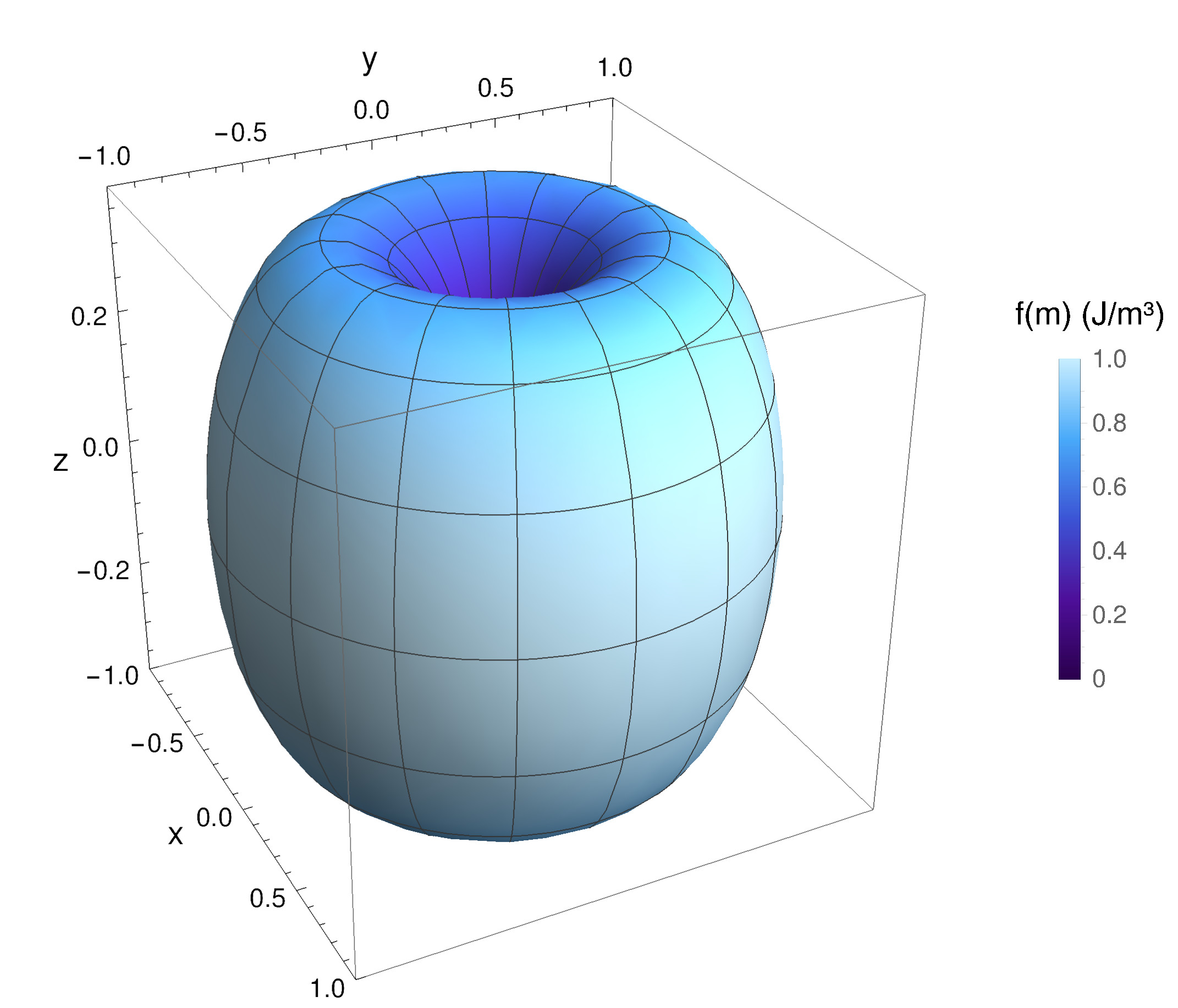
In the case of planar anisotropy, the magnetization prefers to lie in a plane normal to the axis described by the unit vector \(\vb {a}\). The anisotropy energy in this case is
\(\seteqnumber{0}{3.}{20}\)\begin{equation} \mathcal {E}_\text {ani}(\vb {m})=K \, \int _\omega \left (\vb {a}\vdot \vb {m}\right )^2 \dd {\vb {x}} \, . \label {eq:plane_anis} \end{equation}
A visual representation of the energy distribution described by (3.21) is provided in Fig. 3.4. The anisotropy, derived From (3.13), can be expressed as
\(\seteqnumber{0}{3.}{21}\)\begin{equation} \label {eq:hani_plane} \vb {H_\text {ani}}=-\frac {2K}{\mu _0 M_\text {S}}\left (\vb {a}\vdot \vb {m}\right ) \vb {a} \, . \end{equation}
Cubic Anisotropy
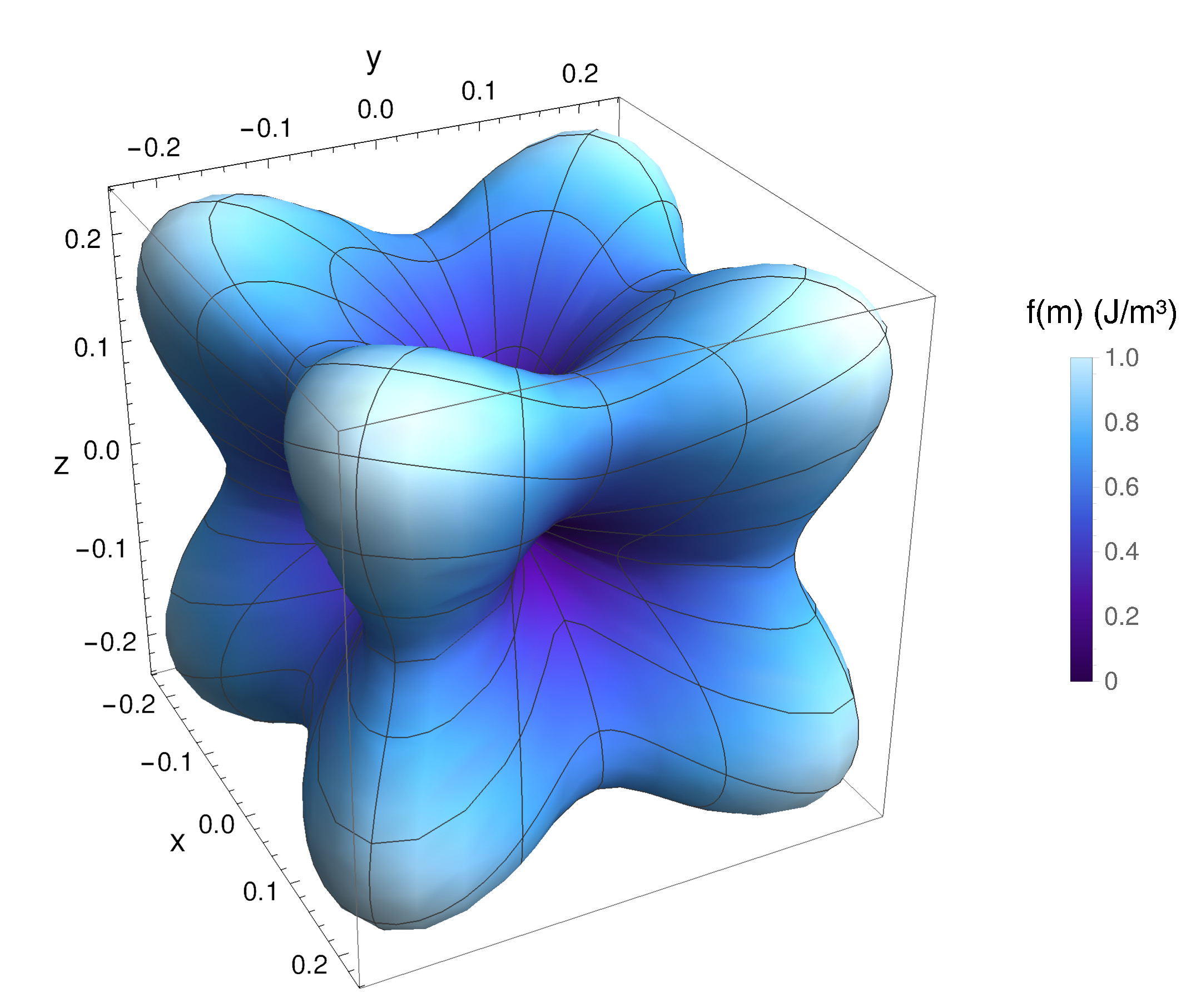
\(+ K_2 \left (\vb {a}_1\vdot \vb {m}\right )^2\left (\vb {a}_2\vdot \vb {m}\right )^2 \left (\vb {a}_3\vdot \vb {m}\right )^2\) representing the cubic anisotropy energy, for \(K_\text {1,2}=1\) J/m\(^3\) and the unit vectors \(\vb {a}_{1}\), \(\vb {a}_{2}\) and \(\vb {a}_{3}\) pointing along the x-, y- and z-axis, respectively. The energy has is minimum value along the x-, y- and z-direction.
In the case of cubic anisotropy, there are three orthogonal preferred orientations for the magnetization, defining three easy axes. These are indicated by the unit vectors \(\vb {a}_1\), \(\vb {a}_2\) and \(\vb {a}_3\). The anisotropy energy can be described by the following expression:
\(\seteqnumber{0}{3.}{22}\)\begin{gather} \nonumber {\mathcal {E}_\text {ani}(\vb {m})=\int _\omega \left \{K_1\left [\left (\vb {a}_1\vdot \vb {m}\right )^2\left (\vb {a}_2\vdot \vb {m}\right )^2 + \left (\vb {a}_1\vdot \vb {m}\right )^2\left (\vb {a}_3\vdot \vb {m}\right )^2 + \left (\vb {a}_2\vdot \vb {m}\right )^2\left (\vb {a}_3\vdot \vb {m}\right )^2\right ] + \right .} \\ \left . K_2 \left (\vb {a}_1\vdot \vb {m}\right )^2\left (\vb {a}_2\vdot \vb {m}\right )^2 \left (\vb {a}_3\vdot \vb {m}\right )^2\right \} \dd {\vb {x}} \label {eq:cube_anis} \end{gather} \(K_1\) and \(K_2\) are anisotropy coefficients specific to the material, which can be positive or negative. A visual representation of the energy distribution described by (3.18) is provided in Fig. 3.5. The cubic anisotropy field in this case is calculated from (3.13) as
\(\seteqnumber{0}{3.}{23}\)\begin{gather} \nonumber \vb {H}_\text {ani} = -\frac {2}{\mu _0 M_S} \left \{ K_1\, \left (\vb {a}_1\vdot \vb {m}\right ) \left (\vb {a}_2\vdot \vb {m}\right ) \left [ \left (\vb {a}_2\vdot \vb {m}\right )\vb {a}_1 + \left (\vb {a}_1\vdot \vb {m}\right )\vb {a}_2 \right ] + \right .\\ \nonumber K_1\, \left (\vb {a}_1\vdot \vb {m}\right ) \left (\vb {a}_3\vdot \vb {m}\right ) \left [ \left (\vb {a}_3\vdot \vb {m}\right )\vb {a}_1 + \left (\vb {a}_1\vdot \vb {m}\right )\vb {a}_3 \right ] + \\ \nonumber K_1\, \left (\vb {a}_2\vdot \vb {m}\right ) \left (\vb {a}_3\vdot \vb {m}\right ) \left [ \left (\vb {a}_3\vdot \vb {m}\right )\vb {a}_2 + \left (\vb {a}_2\vdot \vb {m}\right )\vb {a}_3 \right ] + \\ \nonumber K_2\, \left (\vb {a}_1\vdot \vb {m}\right ) \left (\vb {a}_2\vdot \vb {m}\right ) \left (\vb {a}_3\vdot \vb {m}\right ) \left [ \left (\vb {a}_2\vdot \vb {m}\right )\left (\vb {a}_3\vdot \vb {m}\right )\vb {a}_1 + \right .\\ \left . \left . \left (\vb {a}_1\vdot \vb {m}\right )\left (\vb {a}_3\vdot \vb {m}\right )\vb {a}_2 + \left (\vb {a}_1\vdot \vb {m}\right )\left (\vb {a}_2\vdot \vb {m}\right )\vb {a}_3 \right ] \right \} \, . \label {eq:hani_cubic} \end{gather}
3.2.3 External Field
An external field acts on the magnetization as to have it aligned to itself. The contribution of the external field to the free energy, referred to as Zeeman energy, penalizes deviations of the magnetization from this field throughout the magnetic domain, and can be written as
\(\seteqnumber{0}{3.}{24}\)\begin{equation} \mathcal {E}_\text {ext}(\vb {m}) = -\mu _0 M_\text {S} \int _\omega \vb {H}_\text {ext} \vdot \vb {m} \dd {\vb {x}} \, . \end{equation}
\(\vb {H}_\text {ext}\) denotes the external field expressed in A/m, which can be directly added to the effective field (3.15).
3.2.4 Demagnetizing Field
In a ferromagnetic material, the magnetization itself generates a field contribution to be considered in the effective field, referred to as demagnetizing field, as it acts on the magnetization to reduce its total moment. The related energy contribution, called demagnetization energy, accounts for the dipole-dipole interaction of a magnetic system. Unlike the previously described contributions, the demagnetizing field depends both on the shape of the magnetic domain and on the orientation of the magnetization, acting differently in different structures and geometries, and giving rise to the formation of magnetic domains. Such contribution can be described resorting to the magnetostatic Maxwell equations
\(\seteqnumber{1}{3.26}{0}\)\begin{align} \label {eq:b_expr} \vb {B} & = \mu _0 \left (\vb {H}+M_\text {S}\vb {m}\right ) \, ,\\ \label {eq:div_b} \div {\vb {B}} & = 0 \, ,\\ \label {eq:curl_h} \curl {\vb {H}} & = \vb {J}_\text {C} \, , \end{align} where \(\vb {J}_\text {C}\) is the charge current density. The demagnetizing field generated by the magnetization, noted as \(\vb {H}_\text {demag}\), is only the portion of \(\vb {H}\) independent from electric currents in the system. By putting equations (3.26a) and (3.26b) together, it follows that the demagnetizing field satisfies
\(\seteqnumber{1}{3.27}{0}\)\begin{align} \label {eq:hdemag_div} \div {\vb {H}_\text {demag}} & = -M_\text {S}\div {\vb {m}} \, ,\\ \label {eq:hdemag_curl} \curl {\vb {H}_\text {demag}} & = 0 \, . \end{align} It follows from (3.27b) that \(\vb {H}_\text {demag}\), being a conservative field, can be derived as \(\vb {H}_\text {demag}=-\grad {u}\), where \(u\) is a scalar potential referred to as magnetostatic potential. From (3.27), continuity considerations at the boundary of the magnetic domain and an open boundary condition, it follows that the magnetostatic potential inside the magnetic domain (\(u_\text {in}\)) and outside of it (\(u_\text {out}\)) satisfy the following set of equations:
\(\seteqnumber{1}{3.28}{0}\)\begin{align} -\laplacian {u_\text {in}} & = -M_\text {S}\div {\vb {m}} && \qq {in} \omega \\[6pt] -\laplacian {u_\text {out}} & = 0 && \qq {outside} \omega \\[6pt] \pqty {u_\text {in}-u_\text {out}} & = 0 && \qq {at} \partial \omega \\[6pt] \pqty {\grad {u_\text {in}}-\grad {u_\text {out}}} & = M_\text {S}\,\vb {m}\vdot \vb {n} && \qq {at} \partial \omega \\[6pt] u_\text {out}(\vb {x}) & = \mathcal {O}(1/\abs {\vb {x}}^2) && \qq {as} \vqty {\vb {x}} \rightarrow \infty \end{align} \(\partial \omega \) indicates the external boundary of the magnetic domain, and \(\vb {n}\) is the unit vector normal to the boundary. By referring to the quantities \(-M_\text {S}\div {\vb {m}}\) and \(M_S\,\vb {m}\vdot \vb {n}\) as the volume magnetic charge \(\rho \) and surface magnetic charge \(\sigma \), respectively, the magnetostatic potential can be expressed as [89], [90]
\(\seteqnumber{0}{3.}{28}\)\begin{equation} u(\vb {x}) = \frac {1}{4\pi } \pqty {\int _\omega \frac {\rho (\vb {x}')}{\abs {\vb {x}-\vb {x}'}} \dd {\vb {x}'} + \int _{\partial \omega } \frac {\sigma (\vb {x}')}{\abs {\vb {x}-\vb {x}'}} \dd {\vb {x}'}} \, . \end{equation}
From (3.27a), the demagnetizing field can then be computed as
\(\seteqnumber{0}{3.}{29}\)\begin{equation} \vb {H}_\text {demag}(\vb {x}) = \frac {1}{4\pi } \pqty {\int _\omega \frac {\pqty {\vb {x}-\vb {x}'}\rho (\vb {x}')}{\abs {\vb {x}-\vb {x}'}^3} \dd {\vb {x}'} + \int _{\partial \omega } \frac {\pqty {\vb {x}-\vb {x}'}\sigma (\vb {x}')}{\abs {\vb {x}-\vb {x}'}^3} \dd {\vb {x}'}} \, . \end{equation}
An alternative expression, more convenient for the discretization of the equation using the FD method, can be obtained as the convolution of the magnetization and a kernel representing the dipole interaction [91]:
\(\seteqnumber{0}{3.}{30}\)\begin{equation} \label {eq:hdemag_discr} H_\text {i}^\text {demag}(\vb {x}) = \frac {M_\text {S}}{4\pi } \sum _\text {j} \int _\omega \frac {1}{\abs {\vb {x}-\vb {x}'}^3} \pqty {\frac {x_\text {i} - x_\text {i}'}{\abs {\vb {x}-\vb {x}'}}\frac {x_\text {j} - x_\text {j}'}{\abs {\vb {x}-\vb {x}'}}-\delta _\text {ij}}m_\text {j}(\vb {x}') \dd {\vb {x}'} \end{equation}
\(\text {i,j}=1,2,3\) are the vector components.
The magnetic energy associated with \(\vb {H}_\text {demag}\), usually referred to as magnetostatic energy, can be understood as the energy of the magnetization’s interaction with its own demagnetizing field, and is expressed as
\(\seteqnumber{0}{3.}{31}\)\begin{equation} \mathcal {E}_\text {demag}(\vb {m}) = -\frac {\mu _0 M_\text {S}}{2} \int _\omega \vb {H}_\text {demag}\vdot \vb {m} \dd {\vb {x}} \, . \end{equation}
3.2.5 Ampere Field
When a current is flowing through the magnetic domain, it generates a contribution to the effective field referred to as Ampere field. Looking back at equation (3.26), it can be observed that this field, noted \(\vb {H}_\text {curr}\), is the component of \(\vb {H}\) that satisfies
\(\seteqnumber{1}{3.33}{0}\)\begin{align} \div {\vb {H}_\text {curr}} & = 0 \, ,\\ \curl {\vb {H}_\text {curr}} & = \vb {J}_\text {C} \, . \end{align} Equation (3.33) can be combined with the vector identity
\(\seteqnumber{0}{3.}{33}\)\begin{equation} \curl {\pqty {\curl {\vb {H}_\text {curr}}}} = \grad {\pqty {\div {\vb {H}_\text {curr}}}}-\laplacian {\vb {H}_\text {curr}} \, , \end{equation}
in order to obtain
\(\seteqnumber{0}{3.}{34}\)\begin{equation} \curl {\vb {J}_\text {C}} = \curl {\curl {\vb {H}_\text {curr}}} = -\laplacian {\vb {H}_\text {curr}} \, . \end{equation}
With suitable continuity conditions at the boundary of the magnetic domain and the same open boundary condition considered for the demagnetizing potential, the Ampere field satisfies the following set of equations:
\(\seteqnumber{1}{3.36}{0}\)\begin{align} -\laplacian {\vb {H}_\text {curr}^\text {in}} & = \curl {\vb {J}_\text {e}} && \qq {in} \omega \\[6pt] -\laplacian {\vb {H}_\text {curr}^\text {out}} & = 0 && \qq {outside} \omega \\[6pt] \vb {H}_\text {curr}^\text {in} - \vb {H}_\text {curr}^\text {out} & = 0 && \qq {at} \partial \omega \\[6pt] \pqty {\grad {\vb {H}_\text {curr}^\text {in}}-\grad {\vb {H}_\text {curr}^\text {out}}}\vb {n} & = -\vb {n}\cross \vb {J}_\text {C} && \qq {at} \partial \omega \\[6pt] \vb {H}_\text {curr}^\text {out}(\vb {x}) & = \mathcal {O}(1/\abs {\vb {x}}^2) && \qq {as} \vqty {\vb {x}} \rightarrow \infty \end{align} \(\grad {\vb {H}}\) denotes the vector gradient, with components \(\pqty {\grad {\vb {H}}}_\text {ij} = \pdvline {H_\text {i}}{x_\text {j}}\). A solution for \(\vb {H}_\text {curr}\) consistent with (3.36) is given by Bio-Savart’s law [89]
\(\seteqnumber{0}{3.}{36}\)\begin{equation} \vb {H}_\text {curr} = \frac {1}{4\pi } \int _\omega \vb {J}_\text {C} \cross \frac {\pqty {\vb {x}-\vb {x}'}}{\abs {\vb {x}-\vb {x}'}^3} \dd {\vb {x}'} \, . \end{equation}
The contribution of the Ampere field to the Gibbs free energy is given by
\(\seteqnumber{0}{3.}{37}\)\begin{equation} \mathcal {E}_\text {curr}(\vb {m}) = -\mu _0 M_\text {S} \int _\omega \vb {H}_\text {curr}\vdot \vb {m} \dd {\vb {x}} \, . \end{equation}
3.2.6 Thermal Field
In the presence of a non-zero temperature, the magnetization in a ferromagnet undergoes thermal fluctuations due to heating. The effect of such thermal fluctuations can be described in the LLG formalism by the introduction of an auxiliary random contribution to the effective field, referred to as thermal field. This field must fulfill the following statistical properties [92], [93]:
\(\seteqnumber{1}{3.39}{0}\)\begin{align} \left \langle H_\text {i}^\text {th}(t) \right \rangle & = 0 \\ \left \langle H_\text {i}^\text {th}(t),\,H_\text {j}^\text {th}(t') \right \rangle & = D \, \delta _\text {ij} \, \delta (t-t') \end{align} \(\text {i,j}=1,2,3\) are the spacial coordinates, the constant \(D\) measures the strength of the thermal fluctuations, and \(\langle \,\cdot \,\rangle \) denotes the average taken over different realizations of the stochastic field. Such equations describe a field whose components are uncorrelated in both time and space, and are obtained as random Gaussian distributed numbers with zero mean value. The value of \(D\) is obtained from the Fokker-Planck equation [94]. Given \(\vb {H}_\text {th}\), its contribution to the total Gibbs free energy is given by
\(\seteqnumber{0}{3.}{39}\)\begin{equation} \mathcal {E}_\text {th}(\vb {m}) = -\mu _0 M_\text {S} \int _\omega \vb {H}_\text {th}\vdot \vb {m} \dd {\vb {x}} \, . \end{equation}
3.3 LLG Constraints
As already stated, the LLG equation describes the motion of the magnetization towards a state of minimal energy, described by (3.14). In particular, equation (3.14b) enforces boundary conditions which depend on energy contributions involving spacial derivatives of \(\vb {m}\). The only such term considered throughout this dissertation is the exchange energy, described by (3.16). This term gives rise to the homogeneous Neumann boundary conditions
\(\seteqnumber{0}{3.}{40}\)\begin{equation} \label {eq:bc_llg} \pqty {\grad {\vb {m}}}\vb {n} = \vb {0} \, . \end{equation}
Even though these boundary conditions were derived for the stationary relaxed state, it can be shown that they remain physically valid also in the dynamic case [95], and so they
are usually employed when describing the magnetization dynamics through the LLG equation.
Additionally, the modulus constraint \(\abs {\vb {m}}=1\) introduced in (3.5) must be satisfied. It turns out that, as long as the constraint is satisfied by the initial magnetization, it remains satisfied at any subsequent point in time. To show that, first the scalar product of \(\vb {m}\) with either (3.9), (3.10) or (3.11) is taken, obtaining
\(\seteqnumber{0}{3.}{41}\)\begin{equation} \vb {m}\vdot \pdv {\vb {m}}{t} = 0 \, . \end{equation}
Then, by taking the time derivative of the modulus of \(\vb {m}\) squared, the following expression is derived:
\(\seteqnumber{0}{3.}{42}\)\begin{equation} \pdv {\abs {\vb {m}}^2}{t} = 2\vb {m}\vdot \pdv {\vb {m}}{t} = 0 \end{equation}
It follows that the modulus constraint is always satisfied, provided that it is satisfied by the vector describing the initial magnetization.
3.4 Spin Transfer Torque
The equations discussed up until now allow to describe the magnetization dynamics in the presence of an external field and of contributions internal to the magnetized system. In order to the describe the switching process of an STT-MRAM cell, equation (3.8) must be supplemented with terms describing the spin-transfer torque coming from polarized electrons flowing through the structure. The LLG equation with the addition of this torque contribution takes the form [96], [97]
\(\seteqnumber{0}{3.}{43}\)\begin{equation} \label {eq:gilbert_slonc} \pdv {\vb {m}}{t} = -\gamma _0 \, \vb {m} \times \vb {H}_\text {eff} + \alpha \, \vb {m} \times \pdv {\vb {m}}{t} + \frac {1}{M_\text {S}} \vb {T}_\text {S} \, , \end{equation}
where \(\vb {T}_\text {S}\) is the torque contribution related to the angular momentum transfer between the magnetization and the spin of polarized electrons flowing through the ferromagnetic layers.
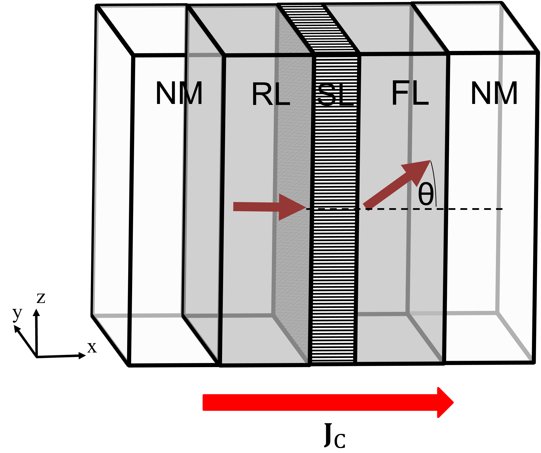
When considering only the torque acting on the free layer of an STT-MRAM cell, schematized in Fig. 3.7, \(\vb {T}_\text {S}\) can be written in terms of the free layer magnetization \(\vb {m}\) and the fixed reference layer magnetization \(\vb {p}\), and is comprised of two contributions, referred to as damping-like and field-like torque [98], [99]:
\(\seteqnumber{0}{3.}{44}\)\begin{equation} \vb {T}_\text {S} = a \, \vb {m}\cross \pqty {\vb {m}\cross \vb {p}} + b \, \pqty {\vb {m}\cross \vb {p}} \end{equation}
\(a\) and \(b\) are parameters depending on the current density flowing through the cell for the damping-like and field-like components, respectively. The damping-like component is the one causing the magnetization of the FL to
move towards the direction of the magnetization of the RL, for AP to P switching, or away from it, for P to AP switching. The field-like component causes a precession of the FL magnetization around the direction of the
magnetization of the RL.
Similarly to (3.11), equation (3.44) can be written in a more numerically tractable form:
\(\seteqnumber{0}{3.}{45}\)\begin{gather} \nonumber {\pdv {\mathbf {m}}{t} = \frac {1}{1+\alpha ^2} \, \bigg \{-\gamma _0 \, \mathbf {m} \times \mathbf {H}_\text {eff} -\gamma _0\alpha \, \mathbf {m} \times \left ( \mathbf {m} \times \mathbf {H_{eff}} \right ) + } \\ \left . - \frac {\gamma \hbar J_\text {C}}{e M_\text {S} d_\text {FL}} \, \eta (\theta ) \, \bqty {\vb {m}\cross \pqty {\vb {m}\cross \vb {p}} - \beta \, \pqty {\vb {m}\cross \vb {p}}}\right \} \label {eq:gilbert_slonc_mod} \end{gather} \(d_\text {FL}\) is the thickness of the free layer, and \(J_\text {C}\) is the modulus of the current density, flowing perpendicular to the structure. \(\eta (\theta )\) is the expression describing the torque efficiency, depending on the relative angle between the magnetization vectors of the free and reference layer \(\theta = \vb {m}\vdot \vb {p}\). \(\beta \) is a coefficient describing the intensity of the field-like torque. When the field-like contribution is not considered, \(\beta =\alpha \). Equation (3.46) is often written by taking the substitution \(\gamma = -g \mu _\text {B}/\hbar \), in the form [92], [93], [100]–[104]
\(\seteqnumber{0}{3.}{46}\)
\begin{gather}
\nonumber {\pdv {\mathbf {m}}{t} = \frac {1}{1+\alpha ^2} \, \bigg \{-\gamma _0 \, \mathbf {m} \times \mathbf {H}_\text {eff} -\gamma _0\alpha \, \mathbf {m} \times \left ( \mathbf {m} \times
\mathbf {H_{eff}} \right ) + } \\ \left . + \frac {g \mu _\text {B} J_\text {C}}{e M_\text {S} d_\text {FL}} \, \eta (\theta ) \, \bqty {\vb {m}\cross \pqty {\vb {m}\cross \vb {p}} - \beta \,
\pqty {\vb {m}\cross \vb {p}}}\right \} \, , \label {eq:gilbert_slonc_mod2}
\end{gather}
where \(g\) is the electron g-factor.
The torque efficiency factor \(\eta (\theta )\) takes different forms for conducting spin-valve structures and MTJs. In the presence of a non-magnetic conducting spacer layer in a symmetric spin-valve, the expression, derived by Slonczewski, is [14]
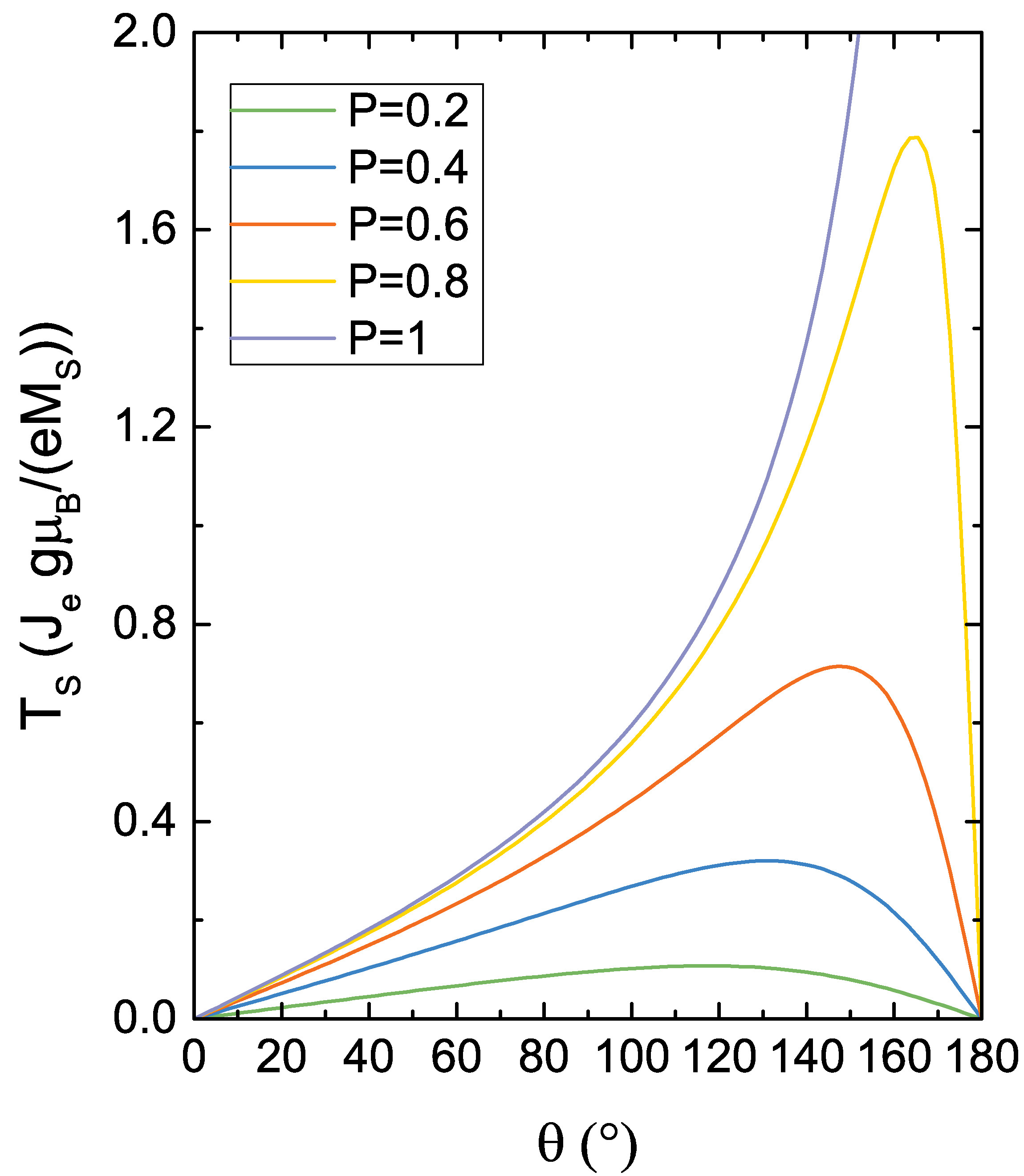
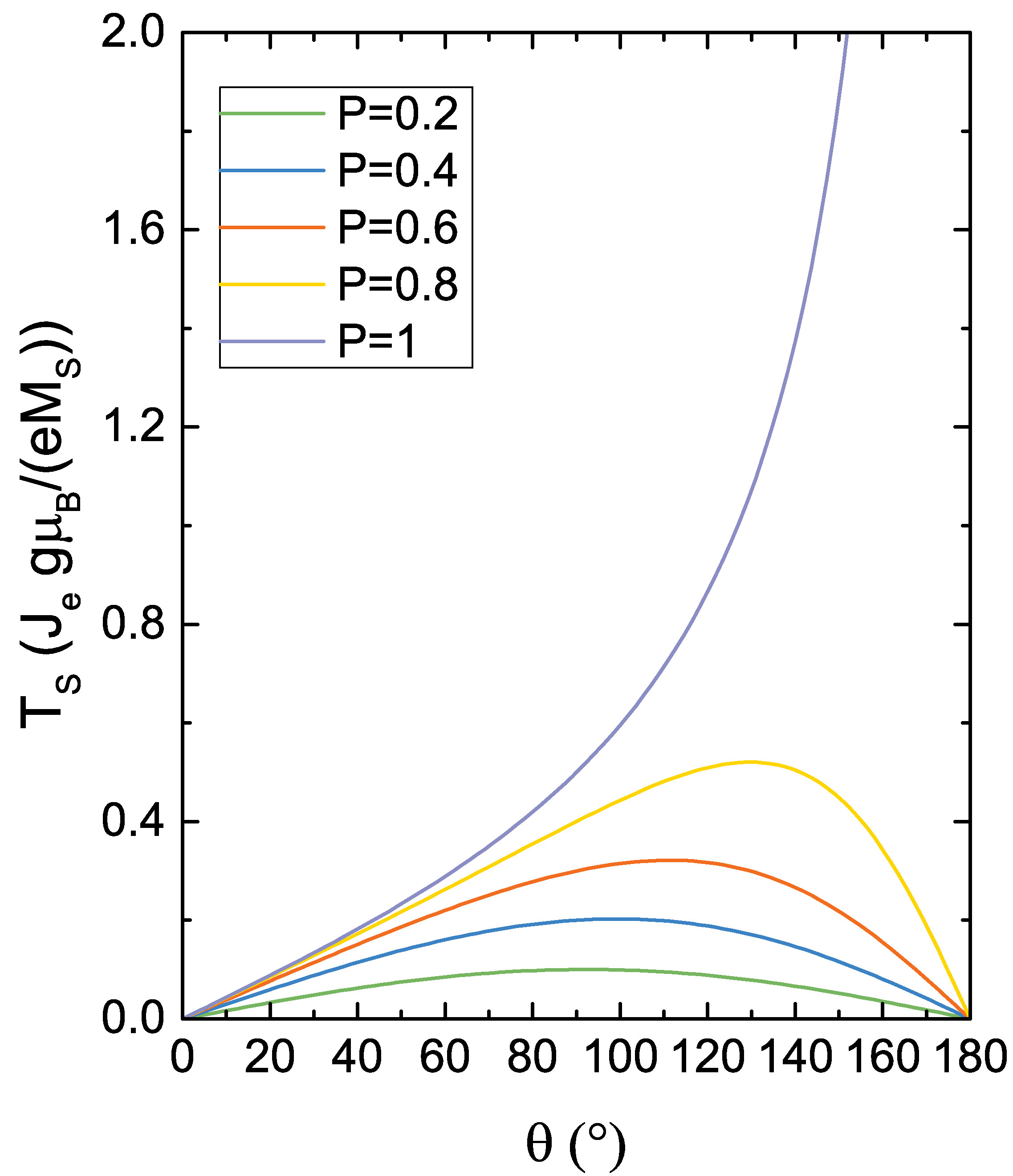
\(\seteqnumber{0}{3.}{47}\)\begin{equation} \label {eq:eta_dep_SV} \eta (\theta ) = \bqty {-4+\pqty {1+P}^3 \, \frac {3+\cos \theta }{4 P^{3/2}}}^{-1} \, . \end{equation}
\(P\) is the polarization factor, taken to be equal in the RL and FL. In the presence of a thin insulating spacer layer in an MTJ, the expression, also derived by Slonczewski, takes the form [16]
\(\seteqnumber{0}{3.}{48}\)\begin{equation} \label {eq:eta_dep_MTJ} \eta (\theta ) = \frac {P}{2 \pqty {1 + P^2 \cos \theta }} \, . \end{equation}
A comparison of the resulting damping-like torque dependence on the angle \(\theta \) between the spin-valve and the MTJ expression, for several values of the polarization parameter \(P\), is reported in Fig. 3.8.
In an MTJ where the RL and the FL have different polarization factors, equation (3.49) for the torque efficiency of the FL can be expressed as
\(\seteqnumber{0}{3.}{49}\)\begin{equation} \label {eq:eta_dep_MTJ_prl} \eta (\theta ) = \frac {P_\text {RL}}{2 \pqty {1 + P_\text {RL}\,P_\text {FL} \cos \theta }} \, , \end{equation}
where \(P_\text {FL(RL)}\) is the polarization of the FL(RL). The torque acting from electrons back-scattering to the RL can be expressed by changing \(P_\text {FL}\) to \(P_\text {RL}\) and vice-versa in the previous expression. The relation between the polarization factors and the TMR can be expressed using Julliere’s formula [16], [99], [105], [106]
\(\seteqnumber{0}{3.}{50}\)\begin{equation} \label {eq:julliere} \text {TMR}=\frac {2\,P_\text {RL}\,P_\text {FL}}{1-P_\text {RL}\,P_\text {FL}} \, . \end{equation}
As previously stated, equations (3.48) and (3.49) are best employed when simulating the magnetization dynamics of a single, thin FL, with a single RL acting as the polarizer. A more general expression for the torque, which allows to deal with an arbitrary number of ferromagnetic and nonmagnetic layers, can be obtained by computing the non-equilibrium spin accumulation in the structure under study, and will be discussed in Chapter 6.