Computation of Torques
in Magnetic Tunnel Junctions

Chapter 4 Charge Current Redistribution and Finite Difference Implementation of the LLG Equation

When dealing with switching simulations of STT-MRAM devices, there can be multiple ways to approach both the evaluation of torques and the evaluation of the current density giving rise to them. This chapter first describes the effects of a high TMR value on the current density distribution in an MRAM cell during switching. This is achieved by deriving an analytical solution for the current density in an MTJ. Then, the FD discretization of the LLG equation employed to perform switching simulations is presented, and is extended with three different approaches to describe the current and its distribution during the switching process.

The magnetization dynamics described by equation (3.47) address the current polarization, giving rise to the STT, via the efficiency terms described by equations (3.48) and (3.49). These terms are based on the theoretical predictions of J. C. Slonczewski, and were derived by considering a macrospin approach to the ferromagnetic leads, where the magnetization in the whole layer can be represented by a single vector. In realistic structures with diameters in the range of tens of nanometers, however, non-uniform switching of the magnetization is expected [107].

In micromagnetic modeling of STT switching, the typical simplified approach is to still rely on the efficiency terms derived by Slonczewski, by using a position dependent angle \(\theta (\vb {r})\) between the magnetization in the RL and FL [17]. Such approach also assumes a position- and time-independent current density \(J_\text {C}\). In circuits, however, the voltage, rather than the current density, remains fixed during switching. The resistance of the tunnel junction depends on the relative magnetization alignment of the FL and the RL, according to (2.4), so the current through the structure is not constant during the process. Moreover, as the magnetization of the FL is not uniform at switching, but depends on the position, so does the local tunneling conductance. The assumption of a constant current density adopted in the description of STT-MRAM switching needs thus to be tested, especially in advanced MTJs with a TMR ratio of about 200% and higher [18].

4.1 Nonuniform Current Density Distribution

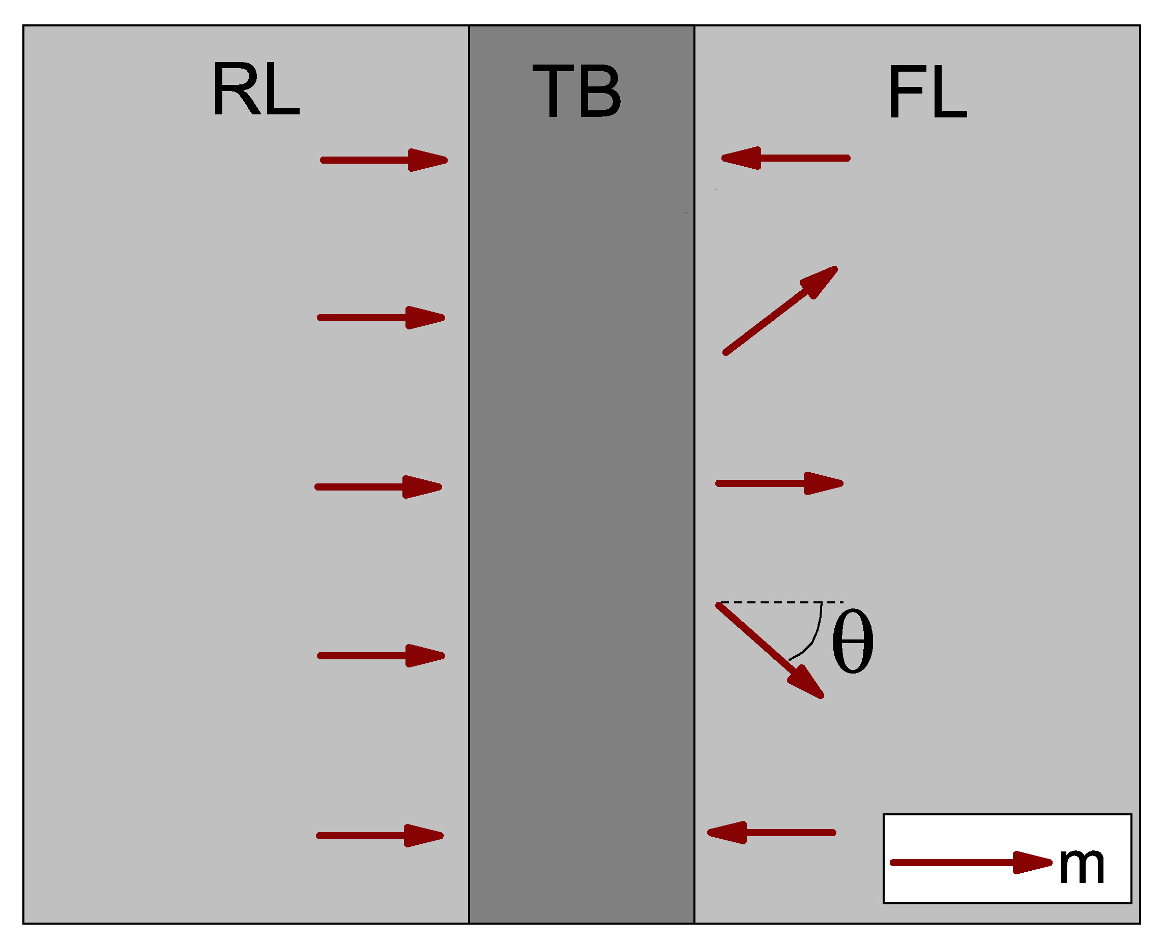
The main effect of a non-uniform magnetization distribution in the FL is to make the resistance of the barrier dependent on the lateral position. The magnitude of the relative resistance variation will be proportional to the TMR of the MTJ. Obtaining a solution for the current density in such a scenario can help evaluate its non-uniformity, and if it needs to be taken into account when performing switching simulations. The MTJ structure in which the current is computed is reported in Fig. 4.1. The considered MTJ has magnetization perpendicular to the plane of the thin ferromagnetic films (p-MTJ), as such structures present better thermal stability and scalability, and lower switching currents (see Chapter 2). The ferromagnetic leads are here contacted directly. The equation for the charge current density in the metallic leads, where the distribution of charges is uniform, is

\begin{equation} \label {eq:metal_curr} \vb {J}_\text {C}=\sigma \vb {E} \, , \end{equation}

where \(\sigma \) is the conductivity, and \(\vb {E}\) is the electric field. In the absence of transient magnetic fields, Maxwell’s equations describe \(\vb {E}\) as an irrotational field, so that in can be written in terms of the electric potential as

\begin{equation} \label {eq:el_field} E=-\grad V \, . \end{equation}

Moreover, the FM layers do not contain sources of electric current, so that

\begin{equation} \label {eq:no_el_sorces} \div {\vb {J}_\text {C}}=0 \, . \end{equation}

As any displacement of the charge density \(n\) relax almost instantly in metals, terms involving its time derivative \(\pdvline {n}{t}\) are hereby not considered. By taking the divergence of both sides of (4.1) and taking (4.2) and (4.3) into consideration, the following Laplace equation for \(V\) can be derived:

\begin{equation} -\sigma \laplacian {V} = 0 \end{equation}

By putting together equations (4.1) and (4.2), the current density can be expressed in terms of the potential as

\begin{equation} \vb {\vb {J}_\text {C}} = -\sigma \grad {V} \, . \end{equation}

To obtain a unique solution for the potential and the current in the FM layers, the boundary conditions need to be defined. Considering the RL, the left side is contacted directly, so that a Dirichlet condition on the voltage, prescribing its value, is applied. The right side of the layer presents the interface with the TB. Here, the tunneling current going to the FL is proportional to the local resistance, which depends on the relative angle between magnetization vectors in the FL and RL, due to the polarized tunneling process in an MTJ, and can be described through equation (2.4). The local resistance of the TB can be modeled through the following Neumann boundary condition, assuming a coordinate system where the x-axis is the one perpendicular to the TB interface:

\begin{equation} \label {eq:voltage_neumann_cond} -\sigma _\text {RL} \grad {V}\vdot \vb {n} = -\sigma _\text {RL} \dv {V}{x}\Bigr |_{\substack {x=t_\text {RL}}} = J_\text {C,TB}(\theta ) \approx \frac {G_\text {MTJ}(\theta )}{S} \Delta V_\text {TB} \end{equation}

\(\sigma _\text {RL}\) is the conductivity of the RL, \(\vb {n}\) is the unit vector normal to the boundary, \(t_\text {RL}\) is the RL thickness, \(J_\text {C,TB}\) is the tunneling spin current density, \(S\) is the TB surface area, and \(\Delta V_\text {TB}\) is the average potential drop across the barrier, computed as the potential on the RL side minus the one on the FL side. The approximate expression for the tunneling current density is justified when the majority of the potential drop across the structure happens at the barrier, so when the resistance of the TB is much higher than the one of the metal contacts. The resistivity of thin films of CoFeB, the most common material for both RL and FL in modern MTJs, is of the order of \(10^{-6}\,\Omega m\) [108], [109]. The typical resistance of an MTJ of \(40\) nm diameter is of the order of \(10\,k\Omega \) [53], giving a resistivity value of about \(10^{-1}\,\Omega m\). Such a resistivity is several orders of magnitude greater then the one of the metal leads, so that the expression for \(J_\text {C,TB}\) is justified.

The solution is first computed for the 2D section of the structure presented in Fig. 4.1, with the x-axis perpendicular to the barrier interface and the y-axis pointing along it. If the angle \(\theta \) entering (4.6) can be described as a function of the position along the TB interface \(y\), then the set of equations describing the potential in the RL layer is

\begin{align} -\pqty {\pdv [2]{V}{x}+\pdv [2]{V}{y}} &= 0 \, ,\\ V(0,y) &= V_0 \, ,\\ \label {eq:bc_laplace_an_2d}\dv {V}{x}\pqty {d_\text {RL},y} &= f(y) \, ,\\ \dv {V}{y}\pqty {x,0} = \dv {V}{y}\pqty {x,w} &= 0 \, . \end{align} \(d_\text {RL}\) and \(w\) are the thickness of the RL and width of the structure, respectively, and the sides of the structure are treated with homogeneous Neumann boundary conditions \(\vb {J_\text {C}}\vdot \vb {n}=0\). In order to solve this set of equations, an explicit expression for the function \(f(y)\), describing a highly nonuniform magnetization distribution, is first provided. The approximate expression for the average voltage drop \(\Delta V_\text {TB}\) in equation (4.6) is obtained by considering the three layers as resistors in series:

\begin{equation} \Delta V_\text {TB} = \frac {R_\text {MTJ}}{R_\text {RL}+R_\text {FL}+R_\text {TB}}\,V_0 \end{equation}

\(R_\text {RL(FL)} = d_\text {RL(FL)}/\pqty {\sigma _\text {RL(FL)}S}\) is the resistance of the RL(FL), and the resistance of the TB is taken as \(R_\text {TB}=S/\int _{S}G_\text {MTJ}(\theta )\dd {S}\). With this expression, boundary condition (4.6) can be rewritten as

\begin{equation} f(y) = -\frac {1}{d_\text {RL}}\frac {R_\text {RL}}{R_\text {RL}+R_\text {FL}+R_\text {TB}}\,V_0\,\pqty {1+\frac {\text {TMR}}{2+\text {TMR}}\cos \theta } \, . \end{equation}

If the unit vector of the RL magnetization is pointing along x, then \(\cos \theta \), being equal to \(\vb {m}_\text {RL}\vdot \vb {m}_\text {FL}\), is equivalent to \(m_\text {x,FL}\). This component of the magnetization is taken to be going from anti-parallel on the sides to parallel in the center of the structure, as \(m_\text {x,FL}(y)=(-1+2\sin \pqty {\pi y/w})\). By taking a TMR value of 200%, the boundary condition (4.7c) can thus finally be written as

\begin{gather} f(y) = -\frac {k_\text {R}}{d_\text {RL}}\,V_0\,g(y) \, ,\\ g(y) = \pqty {\frac {1}{2}+\sin (\frac {\pi y}{w})} \, ,\\ k_\text {R} = \frac {R_\text {RL}}{R_\text {RL}+R_\text {FL}+R_\text {TB}} \, . \end{gather} A solution satisfying (4.7), with the boundary condition (4.10), takes the form

\begin{equation} V\pqty {x,y} = V_0 - \frac {k_\text {R}}{d_\text {RL}}\,V_0\,\pqty {\frac {a_0}{2}\,x + \sum _{n=1}^{\infty } \frac {a_n w}{n \pi \cosh \pqty {\frac {n \pi d_\text {RL}}{w}}} \sinh \pqty {\frac {n \pi x}{w}} \cos \pqty {\frac {n \pi y}{w}}} \, , \end{equation}

where the coefficients \(a_n\) are given by the Fourier cosine series of \(g(y)\):

\begin{equation} g(y) = \frac {a_0}{2} + \sum _{n=1}^{\infty }a_n \cos \pqty {\frac {n \pi y}{w}}\, , \qquad a_n = \frac {2}{w} \int _{0}^{w} g(y) \cos \pqty {\frac {n \pi y}{w}} \dd {y} \end{equation}

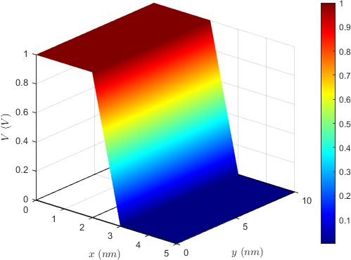
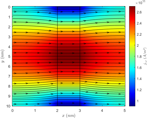
A similar solution can be obtained for the FL, with the Neumann boundary condition applied on its left side instead of the right one, and Dirichlet conditions fixing the potential to 0 on the right side. In the middle layer, a linear decay of the potential from the RL to the FL interface is assumed. The complete solution for both the potential and the current density is reported in Fig. 4.2, for \(\sigma _\text {RL}=\sigma _\text {FL}=10^{6}\) S/m, \(G_0=4.76 \times 10^{-5}\) S, and \(V_0=1\) V. The dimensions of the structure are taken as \(d_\text {RL}=d_\text {FL}=2\) nm and \(w=10\) nm, and the thickness of the TB is \(1\) nm. A voltage drop localized at the TB can be clearly observed in Fig 4.2(a), while the voltage in the two FM contacts is basically constant. The current density profile is reported in Fig. 4.2(b), where the black lines follow the current density vector field. The color bar is based on the magnitude of the x-component of the current. The current density is redistributed to accommodate the conductance variation in the TB, with the percentage difference between the lowest and highest value of the x-component being dictated by the TMR value.

The presented solution can be extended to a three dimensional structure with rectangular cross section. In this case, the partial differential equation to solve for the potential in the RL is

\begin{align} -\pqty {\pdv [2]{V}{x}+\pdv [2]{V}{y}+\pdv [2]{V}{z}} &= 0 \, ,\\ V(0,y,z) &= V_0 \, ,\\ \label {eq:bc_laplace_an_3d}\dv {V}{x}\pqty {d_\text {RL},y,z} &= f(y,z) \, ,\\ \dv {V}{y}\pqty {x,0,z} = \dv {V}{y}\pqty {x,w,z} &= 0 \, ,\\ \dv {V}{y}\pqty {x,y,0} = \dv {V}{y}\pqty {x,y,h} &= 0 \, . \end{align} \(h\) is the height of the structure in the z-direction. Using the same reasoning as before, the boundary condition (4.13c) ca be written as

\begin{gather} \dv {V}{x}\pqty {t_\text {RL},y,z} = -\frac {k_\text {R}}{d_\text {RL}}\,V_0\,g(y,z) \, , \\ g(y,z) = \pqty {\frac {1}{2}+\sin (\frac {\pi y}{w})\sin (\frac {\pi z}{h})} \, .\\ \end{gather} A solution satisfying this set of equations takes the form

\begin{gather} \nonumber {V\pqty {x,y,z} = V_0 - \frac {k_\text {R}}{t_\text {RL}}\,V_0\,\left (\frac {a_{00}}{4}\,x + \sum _{n=1}^{\infty } \frac {a_{n0} w}{2 n \pi \cosh \pqty {\frac {n \pi d_\text {RL}}{w}}} \sinh \pqty {\frac {n \pi x}{w}} \cos \pqty {\frac {n \pi y}{w}} + \right .} \\ \nonumber {+ \sum _{m=1}^{\infty } \frac {a_{0m} h}{2 n \pi \cosh \pqty {\frac {n \pi d_\text {RL}}{h}}} \sinh \pqty {\frac {m \pi x}{h}} \cos \pqty {\frac {m \pi z}{h}} + }\\ \left . + \sum _{n,m=1}^{\infty } \frac {a_{nm}}{ q_{nm} \pi \cosh \pqty {q_{nm} \pi d_\text {RL}}} \sinh \pqty {q_{nm} \pi x} \cos \pqty {\frac {n \pi y}{w}}\cos \pqty {\frac {m \pi z}{h}}\right ) \, , \\ q_{nm} = \sqrt {\pqty {\frac {n\pi }{w}}^2 + \pqty {\frac {m\pi }{h}}^2} \, , \end{gather} where the coefficients \(a_{n,m}\) are again given by the Fourier cosine series for \(g(y,z)\):

\begin{gather} \nonumber {g(y,z) = \frac {a_{00}}{4} + \sum _{n=1}^{\infty }\frac {a_{n0}}{2} \cos \pqty {\frac {n \pi y}{w}} + \sum _{m=1}^{\infty }\frac {a_{0m}}{2} \cos \pqty {\frac {m \pi z}{h}} + } \\ + \sum _{n,m=1}^{\infty }a_{nm} \cos \pqty {\frac {n \pi y}{w}}\cos \pqty {\frac {m \pi z}{h}} \\ a_{nm} = \frac {4}{w\,h} \int _{0}^{w} \dd {y} \int _{0}^{h} \dd {z} g(y,z) \cos \pqty {\frac {n \pi y}{w}} \cos \pqty {\frac {m \pi z}{h}} \end{gather}

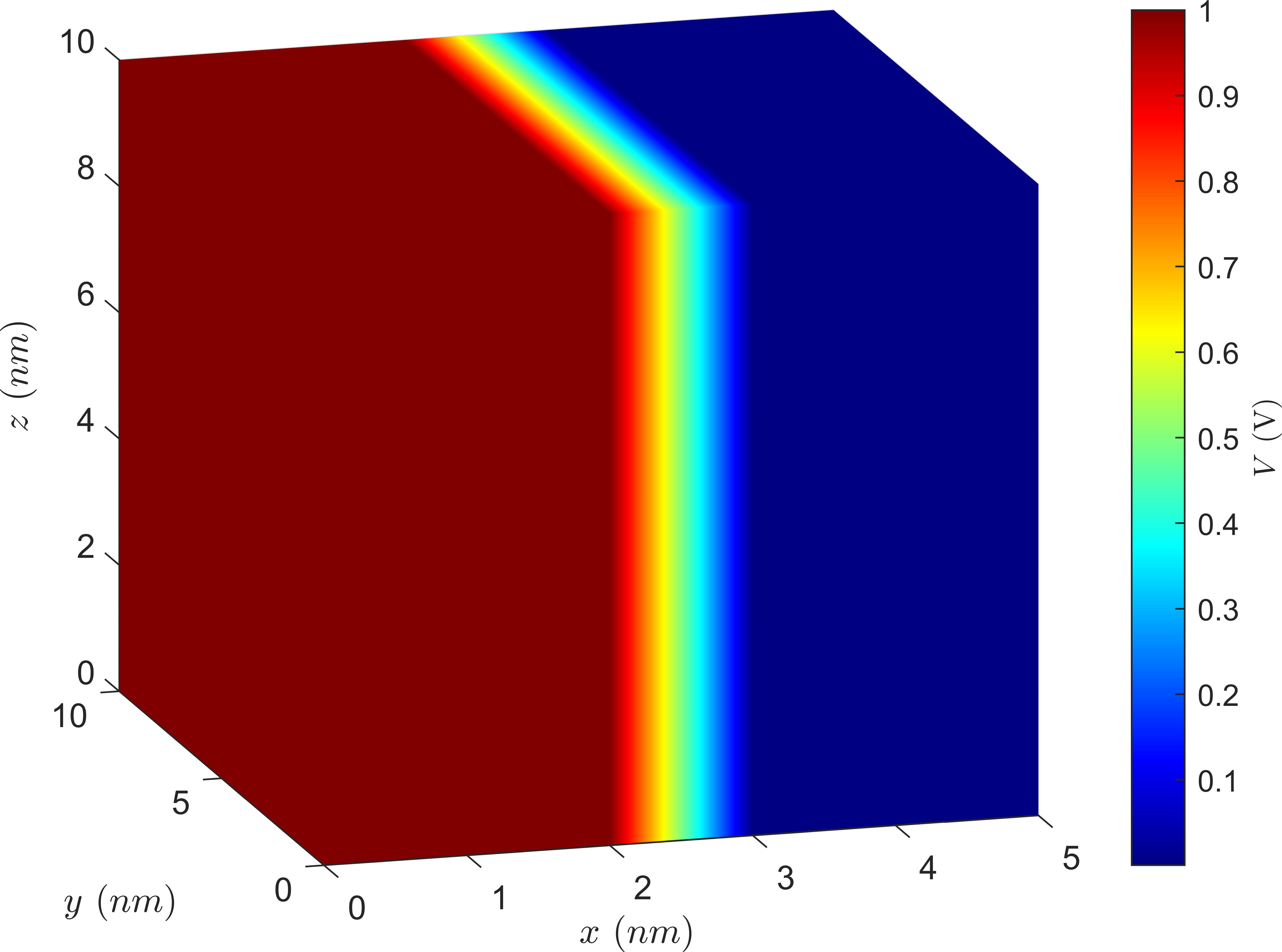
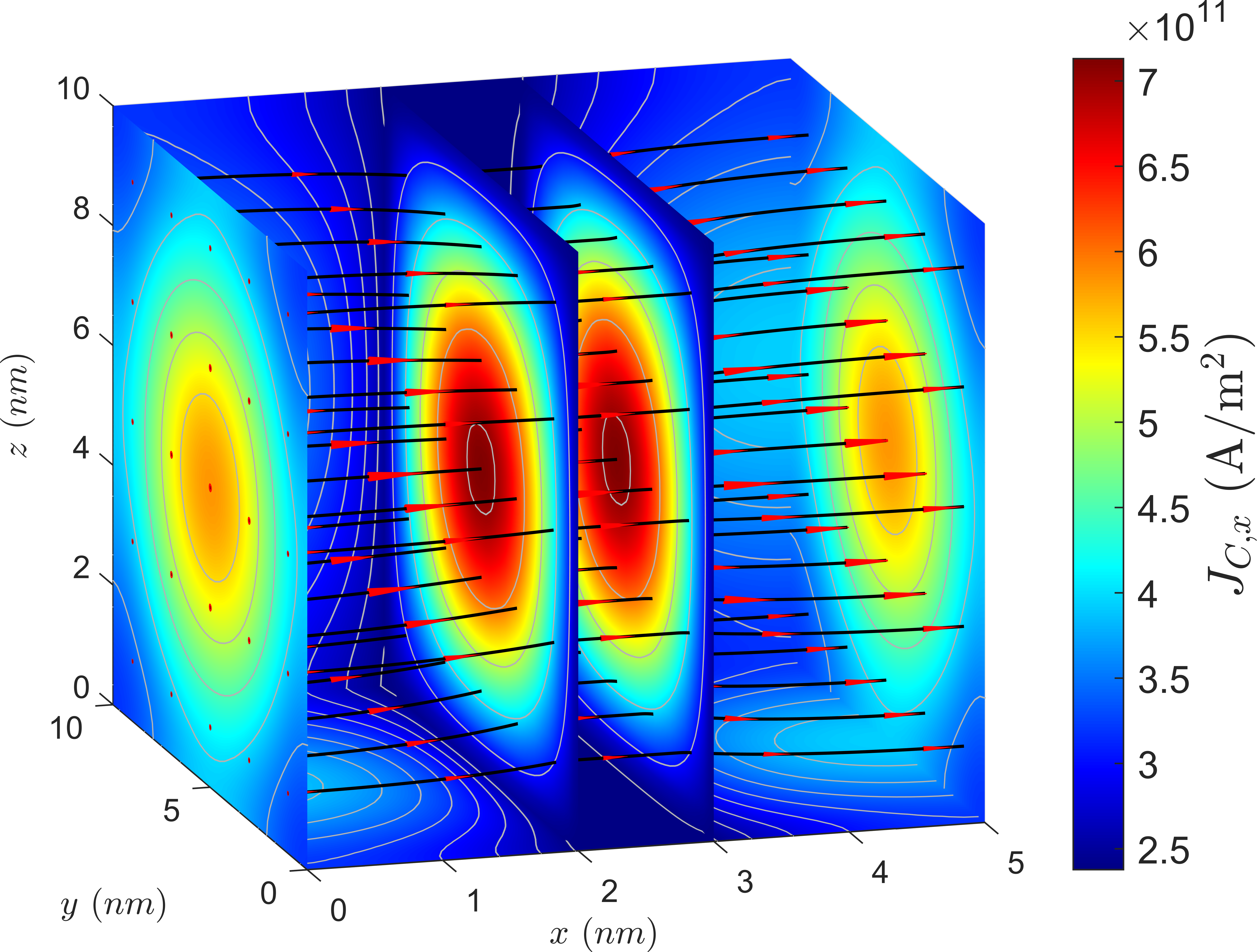
Results for the three-dimensional solution are reported in Fig. 4.3. The distribution of the x-component of the current density is reported for planes located at the contacts and at the TB interfaces. Both the potential and the current density showcase the same behavior reported for the two-dimensional case.

These results underline how the current density component perpendicular to the MTJ plane can be strongly nonuniform when dealing with inhomogeneous magnetization configurations during switching. The validity of the description with the fixed current density for the switching process’ simulation needs thus to be evaluated against models which include the possibility of current density redistribution.

4.2 Finite Difference Implementation of the LLG Equation

The software employed to this end is an in-house solver based on the FD method [17], applied to a pMTJ. The effective magnetic field is calculated directly from the discretized magnetization [91]. Only the dynamics of the FL are computed, while the influence of the RL stray field is added as an external contribution to the effective field. The simulation domain is divided in parallelepiped cells, with volume \(\Delta V=\Delta x \, \Delta y \, \Delta z\), where \(\Delta x\), \(\Delta y\) and \(\Delta z\) represent the discretization along the three Cartesian directions. The number of cells in each direction is labeled \(N_\text {x}\), \(N_\text {y}\) and \(N_\text {z}\), respectively. A unit magnetization vector \(\vb {m}=(m_\text {x}, m_\text {y}, m_\text {z})^T\) is associated with the center of the cell. The software is extended to include the possibility of having several approaches for the local current density computation:

• • an approach where the voltage across the structure is fixed, with the current redistribution exemplified by the results of the previous section;

• • the typical fixed current density approach;

• • an approach with a fixed total current, redistributed according to the local resistance value, extending the reference model described in [111] to pMTJs.

This section provides a brief description of the FD implementation of the terms entering the effective field and torque computation described in chapter 3, as well as the equations employed to address the proposed approaches to the current density redistribution. All the simulations take into account the presence of a single layer of cells along the FL thickness. The labels \(i, j, k\) indicate cells in the three Cartesian directions.

4.2.1 External Field Discretization

A uniform and constant external field vector can be provided as an input parameter to the simulation. Its value is directly added to the effective field vector.

\begin{equation} \label {eq:ext_field_fd} \vb {H_\text {ext}}(i,j,k) = \vb {H_\text {ext,input}} \end{equation}

4.2.2 Exchange Field Discretization

The exchange field contribution, being proportional to the Laplacian of the magnetization, as seen in (3.17), requires knowledge of its value in both the computational cell and its nearest neighbor cells. In the most general case, there are 6 neighbors, two for every Cartesian direction. A first order discretized expression for this contribution takes the form [89]

\begin{equation} \label {eq:exc_field_fd} \vb {H_\text {exc}}(i,j,k) = \frac {2A}{\mu _0 M_\text {S}}\sum _{i',j',k'}\frac {\vb {m}(i',j',k')-\vb {m}(i,j,k)}{\Delta _{i',j',k'}^2} \, . \end{equation}

In this expression, the triplet \((i',j',k')\) describes the nearest neighbors, and can take the forms \((i\pm 1,j,k)\), \((i,j\pm 1,k)\), and \((i,j,k\pm 1)\). \(\Delta _{i',j',k'}\) is the distance between the two magnetization vectors, taking the values \(\Delta x\), \(\Delta y\) and \(\Delta z\) for the different nearest neighbor cells.

The behavior of expression (4.18) at the boundary, where some of the nearest neighbor locations are not part of the simulation domain, needs to be consistent with the boundary condition described by (3.41). The most common way to enforce the given boundary condition is to introduce a ’ghost’ magnetization vector at the missing location, with the same value as the nearest magnetic moment inside the boundary [89]. In the solver, this is achieved by having \(\vb {m}(i',j',k')=\vb {m}(i,j,k)\) for missing neighboring cells.

4.2.3 Magnetocrystalline Anisotropy Field

The computation of the discretized anisotropy field contribution only needs to take into account the magnetization vector in the computational cell. Equations (3.19), (3.22) and (3.24) can be directly employed for the calculation of the field. In the present work, the interface-induced perpendicular anisotropy, typical of pMTJ devices, is modeled as a uniaxial anisotropy contribution. The related discretized expression for the anisotropy field is given by

\begin{equation} \label {eq:hani_uni_fd} \vb {H_\text {ani}}(i,j,k) = \frac {2K}{\mu _0 M_S}\vb {a}\pqty {\vb {m}(i,j,k)\vdot \vb {a}} \, , \end{equation}

where \(\vb {a}\) is the easy axis for the magnetization, taken to be perpendicular to the plane of the structure.

4.2.4 Demagnetizing Field

The demagnetizing field is the most computationally expensive contribution to the effective field. As its origin stems from the dipole interaction, it is a strongly non-local quantity, and its value at a particular location depends on the magnetization vectors in the whole structure. This means that the demagnetizing field calculation in a particular cell requires an iteration over the magnetic moments of all other cells.

For the computation of the demagnetizing field of the FL, a discretization of equation (3.31) is employed. The field for each computational cell is calculated as the sum of the individual demagnetization contributions coming from the magnetic moments of all the cells in the computational domain:

\begin{equation} \label {eq:hdemag_fd} \vb {H_\text {demag}}(i,j,k) = \frac {M_\text {S}}{4\pi }\sum _{i'=1}^{N_\text {x}}\sum _{j'=1}^{N_\text {y}}\sum _{k'=1}^{N_\text {z}} \pqty {\tilde {\vb {G}}(i,j,k,i',j',k')\vb {m}(i',j',k')} \end{equation}

\(\tilde {\vb {G}}\) is a space-dependent matrix describing the dipole-dipole interaction kernel. A detailed derivation of this matrix based on fast calculations of the integrals involved is described in [91]. As the matrix is symmetric, only 6 of its 9 components need to be evaluated. The matrix is also time-independent, so that it can be computed only once at the beginning of the simulation.

The field describing the magnetostatic coupling between RL and FL has the same physical origin of the FL demagnetizing field, but since the magnetization of the RL does not change with time, it can be computed only once at the beginning of the simulation and treated as an external field contribution. In order to compute it, the RL is divided into parallelepiped elementary cells with unit vector magnetization \(\vb {p}=\vb {M_\text {RL}}/M_\text {S,RL}\), where \(\vb {M_\text {RL}}\) is the local magnetization of the RL and \(M_\text {S,RL}\) is its saturation magnetization. An equation similar to (4.20) can be employed for the computation of the magnetostatic contribution:

\begin{equation} \vb {H_\text {ms}}(i,j,k) = \frac {M_\text {S}}{4\pi }\sum _{i'=1}^{N_\text {x,RL}}\sum _{j'=1}^{N_\text {y,RL}}\sum _{k'=1}^{N_\text {z,RL}} \pqty {\tilde {\vb {G}}(i,j,k,i',j',k')\vb {p}(i',j',k')} \end{equation}

\(N_\text {x,RL}\), \(N_\text {y,RL}\) and \(N_\text {x,RL}\) are the number of RL cells in the x-,y-, and z-direction, respectively.

4.2.5 Ampere Field Discretization

A discretized version of equation (3.33) is employed for the computation of the Ampere field. The field acting in each computational cell is obtained by summing the contributions generated by the current density flowing through all the other cells in the simulated domain as

\begin{equation} \vb {H_\text {curr}} = \frac {1}{4\pi }\sum _{i'=1}^{N_\text {x}}\sum _{j'=1}^{N_\text {y}}\sum _{k'=1}^{N_\text {z}} \pqty {\vb {J}_\text {C}(i',j',k') \times \vb {G'}(i,j,k,i',j',k')} \, , \end{equation}

where \(i'\neq i\), \(j'\neq j\), and \(k'\neq k\). \(\vb {J}_\text {C}\) is the current density vector, and \(\vb {G'}\) is a space-dependent vector containing the interaction coefficients between different cells. A detailed description of the derivation of \(\vb {G'}\) based on the fast computation of the integrals involved can be found in [112]. The value of the Ampere field is approximately computed at the beginning of the simulation by assuming a constant current density, and is added to \(\vb {H}_\text {eff}\) as an external field contribution.

4.2.6 Thermal Field Discretization

The implementation of the thermal field must be consistent with (3.39). This can be achieved by computing the thermal field as [113]

\begin{equation} \vb {H_\text {th,l}}(i,j,k) = \sigma (i,j,k)\sqrt {\frac {\alpha }{1+\alpha ^2} \frac {2 k_B T}{\gamma _0 \Delta t \Delta V M_\text {S}}} \, , \end{equation}

where \(l=x,y,z\) is a subscript indicating each thermal field component, \(\Delta t\) is the time-step employed for the simulation and \(\Delta V\) is the volume of a single computational cell. \(\sigma \) is a value generated from a Gaussian distribution uncorrelated in space and time, with standard deviation equal to 1.

4.2.7 Current Density Approaches

The spin-transfer torque term presented in (3.47) can be computed directly from the discretized FL magnetization \(\vb {m}(i,j,k)\) and the RL magnetization \(\vb {p}\), which remains constant during the switching process. The current density \(J_C\) entering the equation, representing the value of the component orthogonal to the TB interface, is given by different expressions, depending on the chosen simulation approach. Noting \(I_\text {C}\) the total current density flowing in the FL, in the fixed voltage approach the expressions for the currents are

\begin{equation} \label {eq:fixed_voltage} V=\text {const} \, , \qquad J_\text {C}(\vb {x},t)=G(\theta (\vb {x},t)) \, \frac {V}{S} \, , \qquad I_\text {C}(t)=\int _{S} J_\text {C}(\vb {x},t) \dd {S} \, . \end{equation}

In the fixed current density approach, they are

\begin{equation} \label {eq:fixed_current_density} J_\text {C}=\text {const} \, , \qquad I_\text {C}=J_\text {C} \, S \, . \end{equation}

Finally, in the fixed total current approach they are

\begin{equation} \label {eq:fixed_total_current} I_\text {C}=\text {const} \, , \qquad J_\text {C}(\vb {x},t)=\frac {G(\theta (\vb {x},t)) \, I_\text {C}}{\int _{S} G(\theta (\vb {x},t)) \dd {S}} \, . \end{equation}

Here, \(S\) is the surface area of the FL, and \(V\) is the applied bias. \(G(\theta )\) is described by equation (2.4) and \(\theta (\vb {x},t)=\vb {m}(\vb {x},t)\vdot \vb {p}\). From these equations, the following discretized expressions for \(J_\text {C}\) in the fixed voltage and fixed current density approaches can be derived:

\begin{align} \text {Fixed Voltage:} \qquad J_\text {C}(i,j,k) &= G(\theta (i,j,1)) \, \frac {V}{S} \\ \text {Fixed Current:} \qquad J_\text {C}(i,j,k) &= \frac {G(\theta (i,j,1)) \, I_\text {C}}{\sum _{i,j,1}G(\theta (i,j,1))\Delta S} \end{align} The conductance \(G\) only depends on the angle \(\theta (i,j,1)=\vb {m}(i,j,1)\vdot \vb {p}\) between the RL magnetization and the FL magnetization in the first layer of cells, closest to the TB, and \(\Delta S\) is the surface area of a single cell.

4.2.8 Time Discretization

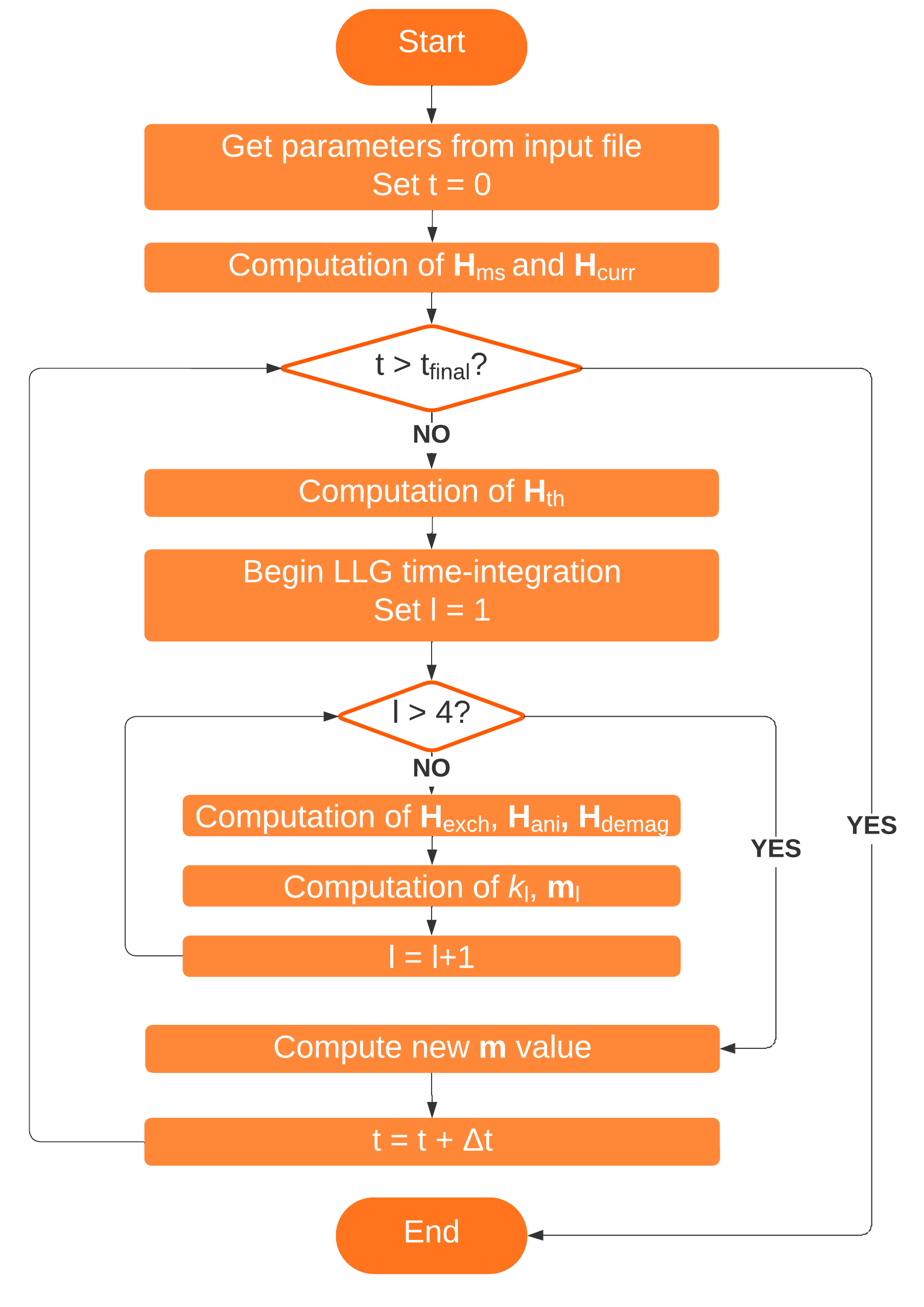
In order to obtain the magnetization dynamics, the LLG equation needs to be integrated over time. The solver employed for this work is based on the fourth-order Runge-Kutta method, with a constant time-step \(\Delta t\). The new value of the magnetization of each cell \(\vb {m}_\text {n+1}=\vb {m}(t_\text {n+1})\), where n is an integer indicating the current time-step and \(t_\text {n+1}=t_\text {n}+\Delta t\), is given by obtaining a weighted average of four increments, where each increment is the product of \(\Delta t\) and an estimated slope specified by the LLG equation at different points of the time-step:

\begin{align} \vb {m}_\text {n+1} &= \vb {m}_\text {n} + \frac {\Delta t}{6}\pqty {k_1 + 2k_2 + 2k_3 + k_4} \\ k_1 &= \text {LLG}\pqty {t_\text {n}, \vb {m}_\text {n}} \\ k_2 &= \text {LLG}\pqty {t_\text {n}+\frac {\Delta t}{2}, \vb {m}_\text {n} + \frac {\Delta t}{2}\,k_1} \\ k_3 &= \text {LLG}\pqty {t_\text {n}+\frac {\Delta t}{2}, \vb {m}_\text {n} + \frac {\Delta t}{2}\,k_2} \\ k_4 &= \text {LLG}\pqty {t_\text {n+1}, \vb {m}_\text {n} + \Delta t\,k_3} \end{align}

The solver implementation and the simulation process are summarized by the flowchart shown in Fig. 4.4.