Computation of Torques
in Magnetic Tunnel Junctions

Chapter 6 Spin and Charge Drift-Diffusion for the Computation of Spin Torques and Finite Element Implementation

The driving factor of the writing process in modern MRAM cells is the torque generated by the polarization process of electrons transiting through the ferromagnetic layers in an MTJ stack. The simulation of the switching process can be achieved by solving the LLG equation for magnetization dynamics, with the inclusion of a term describing the torque acting on the magnetization. As seen in the previous chapters, such term can be defined by employing a Slonczewski-like torque approach [16]. This, however, allows to approximately simulate the magnetization dynamics of a thin free layer only. A more complete description of the process can be obtained by computing the non-equilibrium spin accumulation \(\vb {S}\) across the whole structure. The following sections demonstrate that a more general expression for the torque term \(\vb {T}_\text {S}\) entering (3.44) can be given as [25], [119], [120]

\begin{equation} \label {eq:torque_complete} \vb {T}_\text {S} = -D_\text {e}\frac {\vb {m}\times \vb {S}}{\lambda _{J}^2} - D_\text {e}\frac {\vb {m}\times \pqty {\vb {m}\times \vb {S}}}{\lambda _{\varphi }^2} \, , \end{equation}

where \(D_\text {e}\) is the electron diffusion coefficient. The first term describes precession around the exchange field and is characterized by the exchange length \(\lambda _{J}\), and the second term describes the dephasing process of the spins of the transiting electrons, and is characterized by the dephasing length \(\lambda _\varphi \).

The spin accumulation \(\vb {S}\) describes the deviation of the polarization of the conducting electrons from the equilibrium configuration created by a charge current density \(\vb {J}_\text {C}\), in units of the transported magnetic moment (A/m). Thus, by definition \(\vb {S}\) is non-zero only when an electric current is flowing through the system [83]. A solution for \(\vb {S}\) in all nonmagnetic and ferromagnetic layers of an MRAM cell can be obtained by means of the spin and charge drift-diffusion formalism.

6.1 Spin and Charge Drift-Diffusion

Spin and charge drift-diffusion equations in the presence of a spin-valve structure where the ferromagnetic layers have co-linear (parallel or anti-parallel) magnetization were first derived by T. Valet and A. Fert [121]. A formulation of the equations for the computation of \(\vb {S}\) in the presence of arbitrary magnetization orientation was later reported by S. Zhang, P. Levy and A. Fert [98], and will be hereby summarized. In a magnetic multilayer with the current perpendicular to the plane of the layer, along the x-direction, the linear response of the current to the electric field can be written in spinor form as

\begin{equation} \label {eq:linear_response} \hat {j} = \hat {C}E(x) - \hat {D}\pdv {\hat {n}}{x} \, , \end{equation}

where \(E\) is the electric field, which can be expressed in terms of the electric potential \(V\) as \(E = -\pdvline {V}{x}\), and \(\hat {j}\), \(\hat {C}\), \(\hat {D}\), and \(\hat {n}\) are the \(2\times 2\) spinor matrices representing the current density, the conductivity, the diffusion coefficient, and the accumulation at a given position. For a metal, the diffusion constant and the conductivity are connected via the Einstein relation \(\hat {C}=e^2 \hat {N}_\text {F}\hat {D}\), with \(\hat {N}_\text {F}\) the spin-dependent density of states at the Fermi level. These matrices can in general be expressed in terms of the Pauli matrix vector \(\bm {\sigma }\):

\begin{align} \label {eq:conductivity_expression} \hat {C} &= C_0 \hat {I} + \vb {C}\vdot \hat {\bm {\sigma }} \\ \label {eq:diffusion_expression} \hat {D} &= D_0 \hat {I} + \vb {D}\vdot \hat {\bm {\sigma }} \\ \label {eq:accumulation_expression} \hat {n} &= n_0 \hat {I} + \vb {S}\vdot \hat {\bm {\sigma }} \end{align} \(2 n_0\) is the charge accumulation, \(C_0\) is related to the conductivity \(\sigma \) by \(\sigma =2 C_0\), and \(D_0\) is related to the electron diffusion coefficient by \(D_\text {e} = 2 D_0\). The two vectors \(\vb {C}\) and \(\vb {D}\) are related to the different conductivity and diffusion constant for the majority and minority electrons, labeled \(\sigma ^{\uparrow }\), \(D_\text {e}^{\uparrow }\) and \(\sigma ^{\downarrow }\), \(D_\text {e}^{\downarrow }\), respectively. This difference is characterized by the conductivity polarization parameter \(\beta _\sigma = \pqty {\sigma ^{\uparrow } - \sigma ^{\downarrow }}/\pqty {\sigma ^{\uparrow } + \sigma ^{\downarrow }}\) and the diffusion polarization parameter \(\beta _\text {D} = \pqty {D_\text {e}^{\uparrow } - D_\text {e}^{\downarrow }}/\pqty {D_\text {e}^{\uparrow } + D_\text {e}^{\downarrow }}\). For a transition ferromagnet, \(\vb {C}\) is then defined as \(\vb {C}=\beta _\sigma C_0 \vb {m}\) and \(\vb {D}=\beta _\text {D} D_0 \vb {m}\). The two polarization parameters are different when the density of states for majority and minority electrons is not the same. By inserting (6.3)-(6.5) into (6.2), one obtains the following expressions for the charge current density \(J_\text {C}\) and spin polarization current density \(\vb {J}_\text {S}\) along the x-direction:

\begin{align} J_\text {C} \equiv \text {Re}\pqty {\text {Tr}\bqty {\hat {j}}} &= \sigma E + \frac {e}{\mu _\text {B}} \beta _\text {D} D_\text {e} \pdv {\vb {S}}{x} \vdot \vb {m} \\ \vb {J}_\text {S} \equiv \text {Re}\pqty {\text {Tr}\bqty {\hat {\bm {\sigma }}\hat {j}}} &= -\frac {\mu _\text {B}}{e} \beta _\sigma \vb {m} \sigma E - D_\text {e}\pdv {\vb {S}}{x} \end{align} Terms involving the spatial derivative of the charge accumulation have been ignored, as in metals the distribution of charges can be considered uniform. The factor \(\mu _\text {B}/e\) converts from the units of electric charge, \(A/m^2\), to the ones of the spin polarization current density, \(A/s\). The latter can be converted to the typical units of spin current density by multiplication with the factor \(\hbar /(2\mu _\text {B})\). The spin polarization current density will be referred to as spin current for brevity from now on.

Equation (6.6) only describes the spin and charge currents on the axis perpendicular to a multilayer structure. The generalization to a three-dimensional formulation leads to the following expressions:

\begin{align} \label {eq:3d_charge_current} \vb {J_\text {C}} &= \sigma \vb {E} + \frac {e}{\mu _\text {B}} \beta _\text {D} D_\text {e} \pqty {\grad {\vb {S}}}^\text {T} \vb {m} \\ \label {eq:3d_spin_current} {\tilde {\vb {J}}_\text {S}} &= -\frac {\mu _\text {B}}{e} \beta _\sigma \vb {m} \otimes \pqty {\sigma \vb {E}} - D_\text {e}\grad {\vb {S}} \end{align} \(\otimes \) is the outer product, \(\mathbf {J_C}\) is the charge current density vector, \(\tilde {\vb {J}}_\text {S}\) is the spin current tensor, where the components \(J_\text {S,ij}\) indicate the flow of the i-th component of spin polarization in the j-th direction, and \(\grad {\vb {S}}\) is the vector gradient of \(\vb {S}\), with components \(\pqty {\grad {\vb {S}}}_\text {ij} = \pdvline {S_\text {i}}{x_\text {j}}\). The term \(\pqty {\grad {\vb {S}}}^\text {T}\vb {m}\) is a vector with components \(\pqty {\pqty {\grad {\vb {S}}}^\text {T}\vb {m}}_\text {i} = \sum _\text {j} \pqty {\pdvline {S_\text {j}}{x_\text {i}}} m_j\). In case the current density distribution is known, the spin current can be expressed in terms of the charge current by inserting (6.7a) into (6.7b):

\begin{equation} \label {eq:spin_current_noE} {\tilde {\vb {J}}_\text {S}} = -\frac {\mu _B}{e} \beta _\sigma \vb {m} \otimes \pqty {\vb {J_\text {C}}-\frac {e}{\mu _B} \beta _D D_e \pqty {\grad {\vb {S}}}^\text {T}\vb {m}}-D_e\grad {\vb {S}} \end{equation}

The equation of motion for the spin accumulation in a ferromagnet is determined by the interaction of the local magnetization moment and the spin of the itinerant electrons. This interaction can be described by the Hamiltonian term

\begin{equation} H_\text {int} = -J \vb {S}\vdot \vb {m} \, , \end{equation}

where \(J\) is the coupling strength between local moments and itinerant electrons. The following equation of motion for the spin accumulation can thus be derived:

\begin{equation} \label {eq:spin_accumulation_simple} \dv {\vb {S}}{t}-\frac {J}{\hbar }\vb {m}\times \vb {S}=-\frac {\vb {S}}{\tau _\text {sf}} \end{equation}

\(\tau _\text {sf}\) is the spin-flip relaxation time of the conduction electrons. The second term on the left hand side describes the processional motion of the accumulation due to the exchange interaction. It plays a role when the non-equilibrium spin accumulation and the local magnetization moment are not parallel. The rate of change of \(\vb {S}\) can be expressed in terms of its partial derivative in time and the divergence of the spin current as \(\dv *{\vb {S}}{t}=\pdvline {\vb {S}}{t}+\div {{\tilde {\vb {J}}_\text {S}}}\). By replacing this expression in (6.10), the equation for the spin accumulation becomes

\begin{equation} \label {eq:spin_accumulation_time} \pdv {\vb {S}}{t} = -\div {{\tilde {\vb {J}}_\text {S}}} -D_\text {e}\frac {\vb {S}}{\lambda _{sf}^2}+D_\text {e}\frac {\vb {m}\times \vb {S}}{\lambda _J^2} \, , \end{equation}

where the two length parameters \(\lambda _\text {sf}\) and \(\lambda _\text {J}\) are defined as \(\lambda _\text {sf}=\sqrt {D_\text {e}\tau _\text {sf}}\) and \(\lambda _\text {J}=\sqrt {D_\text {e}\hbar /J}\). \(\div {\tilde {\vb {J}}_\text {S}}\) is the divergence of \(\tilde {\vb {J}}_\text {S}\) with components \(\left (\div {\tilde {\vb {J}}_\text {S}}\right )_\text {i} = \sum _\text {j} \pdvline {J_\text {S,ij}}{x_\text {j}}\).

Equation (6.11) can be further simplified by taking into consideration the fact that the typical time-scales for the spin accumulation and the magnetization are very different. While the former is of the order of picoseconds, the latter is of the order of nanoseconds [98]. For the computation of the spin torque, to be added to the LLG equation (3.44), it is thus sufficient to consider a steady-state expression for the spin accumulation. This assumption was numerically verified in [122]. With \(\pdvline {\vb {S}}{t} = 0\), the equation describing the spin accumulation becomes

\begin{equation} \label {eq:spin_accumulation_nophi} -\div {{\tilde {\vb {J}}_\text {S}}} - D_\text {e}\frac {\vb {S}}{\lambda _{sf}^2} + D_\text {e}\frac {\vb {m}\times \vb {S}}{\lambda _J^2} = 0 \, . \end{equation}

An expression for the torque can be extracted from (6.12) by considering a conservation argument [123]. In the original work of Slonczewski [14], it was argued that the spin current lost by the conducting electrons, described by the divergence term, must have been gained by the magnetization, due to conservation of the total angular momentum. This is always valid in the absence of additional relaxation mechanisms for the spin accumulation [99]. However, in the presence of spin-orbit coupling, part of the angular momentum is transferred to the lattice. This process is responsible for the spin-flip relaxation, described by the \(\lambda _\text {sf}\) term. Spin current lost due to this mechanism does not contribute to the torque acting on the magnetization. The torque can then be obtained as

\begin{equation} \label {eq:torque_incomplete} \vb {T}_\text {S} = -\div {{\tilde {\vb {J}}_\text {S}}} - D_\text {e}\frac {\vb {S}}{\lambda _\text {sf}^2} = -D_\text {e}\frac {\vb {m}\times \vb {S}}{\lambda _J^2} \, . \end{equation}

6.1.1 Spin Dephasing Term

The previous section showed the derivation of a spin torque expression where both the absorption and decay of the transverse spin accumulation components are governed by the exchange length \(\lambda _\text {J}\). Another possible mechanism for the absorption of the transverse components is the dephasing process. Dephasing occurs when, after traveling for a certain distance, different spins have precessed different amounts, so that their transverse components tend to cancel out [120]. In the context of spin transfer torques, this can occur from the variation of electron velocities over the Fermi surface [124] or from spins precessing at the same rate but arriving at different times due to scattering [125]. The behavior of the spin accumulation with both precessional and dephasing terms was described in terms of the Continuous Random Matrix Theory (CRMT) in [125], and the equivalence of CMRT and the spin and charge drift-diffusion formalism was shown. This section gives a brief overview of the derivation thereby presented.

The Landauer-Büttiker formalism, or scattering formalism, is the base for CRMT, and is expressed through a scattering matrix \(S\) relating the initial state and the final state of a physical system undergoing a scattering process [126]. The form of the \(S\) matrix is derived by considering a system where two leads are connected to a central scattering region. The leads are quasi-one-dimensional waveguides. By assuming the solutions to the Schrödinger equation \(\Psi ^\pm _\text {n}=\psi (y)\exp (\pm ik_\text {n}x)\) are known outside of the scattering region, the wave functions \(\Psi ^\pm (x,y)_\text {L/R}\) on the left (L) and right (R) side can be expressed as a linear combination of them:

\begin{equation} \Psi ^\pm (x,y)_\text {L/R} = \sum _{\text {n}} a^\pm _\text {n,L/R}\psi (y)\exp (\pm ik_\text {n}x) \end{equation}

\(\Psi ^+(x,y)_\text {L}\) and \(\Psi ^-(x,y)_\text {R}\) are the incoming wave functions, while \(\Psi ^-(x,y)_\text {L}\) and \(\Psi ^+(x,y)_\text {R}\) are the outgoing wave functions. By expressing the vectors containing the expansion coefficients \(a^\pm _\text {n,L/R}\) as \(\Psi ^\pm _\text {L/R}\), the incoming and outgoing vectors can be related by a matrix \(S\) composed of reflection (\(r,r'\)) and transmission (\(t,t'\)) submatrices:

\begin{gather} \begin{pmatrix} \Psi ^-_\text {L} \\ \Psi ^+_\text {R} \end {pmatrix} = \begin{pmatrix} r' & t \\ t' & r \end {pmatrix} \begin{pmatrix} \Psi ^+_\text {L} \\ \Psi ^-_\text {R} \end {pmatrix} ,\qquad \begin{pmatrix} r' & t \\ t' & r \end {pmatrix} =S \end{gather} If two conductors A and B described by this scattering formalism are in series, the transmission and reflection of the whole system can be written as

\begin{gather} \label {eq:trans_refl_sum} t_\text {AB}=t_\text {B}\frac {1}{1-r_\text {A}r'_\text {B}}t_\text {A} \, , \\ r_\text {AB}=r_\text {B} + t_\text {B}\frac {1}{1-r_\text {A}r'_\text {B}}r_\text {A}t'_\text {B} \, . \end{gather} The conductance of a system can be expressed in terms of its transmission matrix \(t\) as

\begin{equation} G = \frac {e^2}{h} \text {T}\, , \qquad \text {T} = \text {Tr}\bqty {tt^\dagger } \, . \end{equation}

The value \(\text {T}\) corresponds to the sum over the probabilities of being transmitted from one side of the system to the other, and \(h\) is the Planck constant. The same expression holds true for the reflection probabilities, represented by the quantity \(\text {R}=\text {Tr}\bqty {rr^\dagger }\). By taking a semi-classical limit and assuming that successive reflections mix together different channels, it can be assumed that each electron traveling through the system picks up a certain phase. The transmission through the whole system takes then the form

\begin{equation} t_\text {AB}=t_\text {B}\frac {1}{1-\abs {r_\text {A}r'_\text {B}}z}t_\text {A} \, , \end{equation}

where \(z=\exp (i\varphi )\) describes the phase acquired by the traveling electrons. An expression for the conductance is obtained by taking the average over all values of \(\varphi \):

\begin{equation} \langle G_\text {AB} \rangle = \frac {e^2}{h} \langle \text {T}_\text {AB} \rangle \end{equation}

The average value can be computed through the residual theorem by integrating over the phase in the complex space. This leads to the expression

\begin{equation} \langle \text {T}_\text {AB} \rangle = \text {T}_\text {B}\frac {1}{1-\text {R}_\text {A}\text {R}'_\text {B}}\text {T}_\text {A} \, , \label {eq:trans_refl_prob_sum} \end{equation}

which has the same form of (6.16a), but it relates probabilities instead of amplitudes. The same is also true for the quantity \(\langle \text {R}_\text {AB} \rangle \). This means that, within the semi-classical limit, transport can be described by a scattering-like formalism concerning only probabilities.

The same theoretical description, employed until now only in the presence of multiple channels, can also be applied in the presence of the additional spin degree of freedom. In this case, the transmission and reflection matrices have dimensions of \(4N_\text {ch} \times 4N_\text {ch}\), with \(N_\text {ch}\) the number of channels. The random matrix theory (RMT) employed in [126] can be applied to account for both mixing of the contributions in different channels and loss of coherence of the waves traveling through the system, in a similar fashion to the average over the phase previously shown. The resulting theory presents a structure similar to the scattering formalism, with \(4 \times 4\) spin-dependent transmission and reflection matrices, indicated by a hat. The block matrix \(\hat {S}\) describing transport through a conductor takes the form

\begin{equation} \label {eq:Shat} \hat {S} = \begin{pmatrix} \hat {r}' & \hat {t} \\ \hat {t}' & \hat {r} \end {pmatrix} \, . \end{equation}

Each of the four submatrices is defined from the \(4N_\text {ch} \times 4N_\text {ch}\) matrices of the scattering theory, relating different spins and channels, by the following expression:

\begin{equation} \hat {t}_{\sigma \eta , \sigma ' \eta '} = \frac {1}{N_\text {ch}} \text {Tr}_{N_\text {ch}}\bqty {t_{\sigma \eta } t^\dagger _{\sigma ' \eta '}} \end{equation}

\(\sigma \) and \(\eta \) indicate the up (\(\uparrow \)) or down (\(\downarrow \)) spin orientation. Similar expressions hold for the other transmission and reflection matrices. The most important contributions to the obtained matrix are the probabilities \(\text {T}_{\sigma \eta }=\hat {t}_{\sigma \eta , \sigma \eta }\) and the mixing coefficients \(\text {T}_\text {mx}=\hat {t}_{\sigma \sigma , -\sigma -\sigma }\). The other entries in the matrix have a negligible contribution to the overall transport description and can be disregarded [126]. The final form of the \(\hat {t}\) matrix is then given by

\begin{equation} \hat {t} = \begin{pmatrix} \text {T}_{\uparrow \uparrow } & 0 & 0 & \text {T}_{\uparrow \downarrow } \\ 0 & \text {T}_\text {mx} & 0 & 0 \\ 0 & 0 & \text {T}^*_\text {mx} & 0 \\ \text {T}_{\downarrow \uparrow } & 0 & 0 & \text {T}_{\downarrow \downarrow } \end {pmatrix} \, . \end{equation}

Similar expressions hold true for the other matrices entering (6.21). The coefficients \(\text {T}_{\sigma \eta }=\hat {t}_{\sigma \eta , \sigma \eta }\) describe the probability of an electron with spin \(\sigma \) to be transmitted with spin \(\eta \). The mixing coefficients are related to the precession and loss of coherence of electrons with a spin non-colinear with the magnetization:

\begin{equation} \label {eq:transverse_transmission} \text {T}_\text {mx} \approx \exp (-d/l_\perp + id/l_\text {L}) \end{equation}

\(d\) is the thickness of the ferromagnetic conductor, and \(l_\text {L}\) is the Larmor precession length. The term containing \(l_\perp \) is related to the fact that the amount of precession depends on the direction of incidence of the electron into the ferromagnet. Two electrons with different incidence angles will undergo a dephasing process. This results is an exponentially decaying spin density orthogonal to the local magnetization which absorbs the transverse components of the spin current. \(l_\perp \) indicates the typical length over which these absorption process occurs.

Most of the quantities described until now can be recast in terms of semi-classical properties. The conductance can now be expressed as

\begin{equation} G = \pqty {\text {T}_{\uparrow \uparrow } + \text {T}_{\uparrow \downarrow } + \text {T}_{\downarrow \uparrow } + \text {T}_{\downarrow \downarrow }}/R_\text {sh} \, , \end{equation}

where \(R_\text {sh}=h/\pqty {e^2 N_\text {ch}}\) is the Sharvin resistance. It corresponds to the resistance of a perfectly transparent waveguide, with \(N_\text {ch}\) propagating transversal modes. As shown in [126], the addition laws for transmission and reflection in equation (6.20) are still valid. Moreover, it is shown that the number of degrees of freedom can be reduced from the incoming and outgoing wave function coefficients to vectors of length 4, storing only the charge and spin degrees of freedom. These vectors are noted \(P^\pm _\text {4,L/R}\), and the incoming and outgoing vectors are related through the \(\hat {S}\) matrix (6.21) as

\begin{equation} \label {eq:PShat} \begin{pmatrix} P^-_\text {4,L} \\ P^+_\text {4,R} \end {pmatrix} = \hat {S} \begin{pmatrix} P^+_\text {4,L} \\ P^-_\text {4,R} \end {pmatrix} \, . \end{equation}

As shown in [125], one can demonstrate the equivalence of the random matrix description to the spin and charge drift-diffusion formalism. First, transport in a discretized one-dimensional conductor, divided into \(N\) parts, is considered. The \(P_\text {4}\) vectors of each part can be related through the node equations

\begin{align} P^+_\text {4,L}\bqty {i+1} &= P^+_\text {4,R}\bqty {i} \, , \\ P^-_\text {4,L}\bqty {i+1} &= P^-_\text {4,R}\bqty {i} \, , \end{align} where \(i\) is an index going from \(1\) to \(N\). Through a variable change, the \(P_\text {4}\) vectors can be employed to obtain the four dimensional potential \(\mu _\text {4}\) and current \(j_\text {4}\) in the system [127]:

\begin{gather} \mu _\text {4} = \frac {1}{2}\pqty {P^+_\text {4,L}+P^-_\text {4,L}} \\ j_\text {4} = \frac {1}{2}\pqty {P^+_\text {4,L}-P^-_\text {4,L}} \end{gather} After the change of variables, and by assuming that transmission and reflection properties do not depend on the direction, equations (6.26) and (6.27) can be combined to obtain the following relations:

\begin{align} 2\pqty {\mu _\text {4}\bqty {i+1} - \mu _\text {4}\bqty {i}} &= \pqty {\hat {r} - \hat {t} + 1}\pqty {\mu _\text {4}\bqty {i+1} - \mu _\text {4}\bqty {i} - j_\text {4}\bqty {i+1} - j_\text {4}\bqty {i}} \\ 2\pqty {j_\text {4}\bqty {i+1} - j_\text {4}\bqty {i}} &= \pqty {\hat {r} + \hat {t} - 1}\pqty {\mu _\text {4}\bqty {i+1} + \mu _\text {4}\bqty {i} - j_\text {4}\bqty {i+1} + j_\text {4}\bqty {i}} \end{align}

In order to go from the discrete description presented until now to a continuous one which recovers the drift-diffusion formalism, one must go to the limit where the length of each material slice goes to the infinitesimal quantity \(\dd {x}\). This gives the possibility of describing the thin slices’ \(\hat {S}\) matrix components with the following parametrization [128]:

\begin{align} \hat {t} &= 1-\Lambda _\text {t}\dd {x} \\ \hat {r} &= \Lambda _\text {r}\dd {x} \end{align} \(\Lambda _\text {t}\) and \(\Lambda _\text {r}\) are \(4 \times 4\) matrices. These expressions can be inserted back into equation (6.29), to obtain the following formulation:

\begin{align} 2\pqty {\mu _\text {4}\pqty {x+\dd {x}} - \mu _\text {4}\pqty {x}} &= \dd {x} \pqty {\Lambda _\text {r} + \Lambda _\text {t}}\pqty {\mu _\text {4}\pqty {x+\dd {x}} - \mu _\text {4}\pqty {x} - j_\text {4}\pqty {x+\dd {x}} - j_\text {4}\pqty {x}} \\ 2\pqty {j_\text {4}\pqty {x+\dd {x}} - j_\text {4}\pqty {x}} &= \dd {x} \pqty {\Lambda _\text {r} - \Lambda _\text {t}}\pqty {\mu _\text {4}\pqty {x+\dd {x}} + \mu _\text {4}\pqty {x} - j_\text {4}\pqty {x+\dd {x}} + j_\text {4}\pqty {x}} \end{align} The equations can then be developed to the first order in \(\dd {x}\) to obtain the continuous differential equations

\begin{align} -\pdv {\mu _\text {4}}{x} \pqty {x} &= 2 \Lambda _\Omega j_\text {4}(x) \, ,\\ -\pdv {j_\text {4}}{x} \pqty {x} &= 2 \Lambda _\Xi \mu _\text {4}(x) \, , \end{align} where \(2\Lambda _\Omega = \Lambda _\text {t}+\Lambda _\text {r}\) and \(2\Lambda _\Xi = \Lambda _\text {t}-\Lambda _\text {r}\). These matrices, defined so that they fit the Valet-Fert theory, take the form

\begin{align} \Lambda _\Omega &= \begin{pmatrix} \Gamma _{\uparrow } & 0 & 0 & 0 \\ 0 & \Gamma _\text {mx,eff} & 0 & 0 \\ 0 & 0 & \Gamma ^*_\text {mx,eff} & 0 \\ 0 & 0 & 0 & \Gamma _{\downarrow } \end {pmatrix} \, , \\ \Lambda _\Xi &= \begin{pmatrix} \Gamma _\text {sf} & 0 & 0 & -\Gamma _\text {sf} \\ 0 & \Gamma _\tau & 0 & 0 \\ 0 & 0 & \Gamma ^*_\tau & 0 \\ -\Gamma _\text {sf} & 0 & 0 & \Gamma _\text {sf} \end {pmatrix} \, . \end{align} The coefficients of these two matrices are linked to the characteristic length scales of the material. \(\Gamma _{\uparrow (\downarrow )}=1/l_{\uparrow (\downarrow )}\) is the mean free path for majority (minority) electrons. It can be rewritten in terms of the mean free path \(l_*=\pqty {1/l_{\uparrow }+1/l_{\downarrow }}^{-1}\) and spin asymmetry of the material \(\beta \), introduced by Valet-Fert in [121] as \(\Gamma _{\uparrow (\downarrow )} = (1 \mp \beta )/(2 l^*)\). These length scales are connected to the spin-dependent resistivities of the Valet-Fert theory [121] as \(l_{\uparrow (\downarrow )}=R_\text {sh}/\rho _{\uparrow (\downarrow )}\) and \(l_*=R_\text {sh}/(4\rho _*)\). \(\Gamma _\text {mx,eff}=\Gamma _\text {mx}/2+\pqty {\Gamma _{\uparrow }+\Gamma _{\downarrow }}/2\) is the component describing the behavior of the electrons with spin direction transverse to the local magnetization. \(\Gamma _\text {mx}=1/l_\perp -i/l_\text {L}\) is of ballistic origin, and describes the spin-dependent part of the transport, with the Larmor precession length and spin penetration length introduced in (6.24). The second part is related to the spin-independent part of the transport. \(\Gamma _\text {sf}=l_*/(4 l_\text {sf}^2)\) is connected to spin-flip processes, and \(l_\text {sf}\) is referred to as spin diffusion length. Finally, \(\Gamma _\tau =\Gamma _\text {mx}/2+2\Gamma _\text {sf}\) describes the behavior of the non-conserved part of the transverse spins, including the fact that they are also affected by spin-flip processes.

It is then possible to recover charge and spin potentials (\(\mu _\text {c}\) and \(\bm {\mu }\), respectively) and charge and spin currents (\(j_c\) and \(\vb {j}\), respectively) from the variables \(\mu _\text {4}\) and \(j_\text {4}\). The process, described in detail in [125], involves a change of basis based on the set of \(4 \times 4\) matrices \(\text {I}_\text {ij}=\sigma _\text {i} \otimes \sigma ^*_\text {j}\), where \(i,j=0,1,2,3\), \(\sigma _0\) is the identity matrix and \(\sigma _{1,2,3}\) are the Pauli matrices. The resulting equations can be expressed in the same units employed for the Zhang-Levi-Fert formalism (6.6) through a change of variables. All the potentials and currents described until now are expressed in units of energy. One can express the charge potentials in units of V as \(V=e\mu _\text {c}\) and convert the spin potential to spin accumulation, expressed in units of A/m, as \(\vb {S} = -\pqty {\mu _\text {B}\sigma / \pqty {e^2 D_\text {e}}} ~ \bm {\mu }\) [83]. The charge current expressed in the usual units of A/m\(^2\) is \(J_\text {C} = \pqty {e/\pqty {4 R_\text {sh}}} ~ j_\text {c}\), and the spin polarization current density, expressed in units of \(A/s\), is \(\vb {J}_\text {S}=-\pqty {4\mu _\text {B} / \pqty {e^2 R_\text {sh}}} ~ \vb {j}\) [83], [123]. Furthermore, the relations between the Zhang-Levy-Fert and Valet-Fert theories derived in [83] can be extended to include the length scales coming from the CMRT derivation:

\begin{align} \sigma &= \frac {1}{\rho _* \pqty {1-\beta ^2}} \\ \lambda _\text {sf}^2 &= \frac {l_\text {sf}^2}{1-\beta ^2} \\ \lambda _\text {J}^2 &= \frac {l_* l_\text {L}}{1-\beta ^2} \\ \lambda _{\varphi }^2 &= \frac {l_\perp }{l_\text {L}} \lambda _{J}^2 \\ \lambda ^2 &= \frac {l_*^2}{1-\beta ^2} \end{align} \(\lambda _{\varphi }\) is the spin dephasing length introduced in (6.1), \(\lambda =\sqrt {D_\text {e} \tau }\) is the momentum relaxation length, and \(\tau \) is the time for momentum relaxation [98], [129]. The spin asymmetry parameter \(\beta \) of the Valert-Fert model is equivalent to the conductivity polarization \(\beta _\sigma \) in the Zhang-Levy-Fert approach. Finally, the spin and charge drift-diffusion equations for transport along the x-direction obtained through the formalism of [125] are, after the change of variables:

\begin{gather} J_\text {C} = \sigma E + \frac {e}{\mu _\text {B}} \beta _\text {D} D_\text {e} \pdv {\vb {S}}{x} \vdot \vb {m} \\ \vb {J}_\text {S} - \frac {\lambda ^2}{\lambda _J^2} \vb {m} \times \vb {J}_\text {S} - \frac {\lambda ^2}{\lambda _\varphi ^2} \vb {m} \times \pqty {\vb {m} \times \vb {J}_\text {S}} = -\frac {\mu _\text {B}}{e} \beta _\sigma \vb {m} \sigma E - D_\text {e}\pdv {\vb {S}}{x} \\ \pdv {J_\text {C}}{x} = 0 \\ -\pdv {\vb {J}_\text {S}}{x} - D_\text {e} \frac {\vb {S}}{\lambda _{sf}^2} + D_\text {e} \frac {\vb {m} \times \vb {S}}{\lambda _{J}^2} + D_\text {e} \frac {\vb {m} \times \pqty {\vb {m} \times \vb {S}}}{\lambda _{\varphi }^2} = 0 \end{gather} A generalization of these equations to three-dimensions leads to the following expressions [119], [123], [125]:

\begin{gather} \vb {J}_\text {C} = \sigma \vb {E} + \frac {e}{\mu _\text {B}} \beta _\text {D} D_\text {e} \pqty {\grad {\vb {S}}}^\text {T} \vb {m} \label {eq:3d_dd_luc_charge_curr}\\ {\tilde {\vb {J}}_\text {S}} - \frac {\lambda ^2}{\lambda _J^2} \bqty {\vb {m}}_\times {\tilde {\vb {J}}_\text {S}} - \frac {\lambda ^2}{\lambda _\varphi ^2} \bqty {\vb {m}}_{\times \times } {\tilde {\vb {J}}_\text {S}} = -\frac {\mu _\text {B}}{e} \beta _\sigma \vb {m} \otimes \pqty {\sigma \vb {E}} - D_\text {e}\grad {\vb {S}} \label {eq:3d_dd_luc_spin_curr} \\ \div {\vb {J}_\text {C}} = 0 \label {eq:3d_dd_luc_charge_pot} \\ -\div {{\tilde {\vb {J}}_\text {S}}} - D_\text {e} \frac {\vb {S}}{\lambda _{sf}^2} + D_\text {e} \frac {\vb {m} \times \vb {S}}{\lambda _{J}^2} + D_\text {e} \frac {\vb {m} \times \pqty {\vb {m} \times \vb {S}}}{\lambda _{\varphi }^2} = 0 \label {eq:3d_dd_luc_soin_acc} \end{gather} \(\bqty {\vb {m}}_{\times }\) and \(\bqty {\vb {m}}_{\times \times }\) indicate the matrices associated with the cross-product and double cross-product with \(\vb {m}\):

\begin{equation} \bqty {\vb {m}}_{\times } = \begin{pmatrix} 0 & -m_\text {1} & m_\text {2} \\ m_\text {3} & 0 & -m_\text {1} \\ -m_\text {2} & m_\text {1} & 0 \\ \end {pmatrix}, \,\, \bqty {\vb {m}}_{\times \times } = \begin{pmatrix} -m_\text {2}^2 - m_\text {3}^2 & m_\text {1} m_\text {2} & m_\text {1} m_\text {3} \\ m_\text {1} m_\text {2} & -m_\text {1}^2 - m_\text {3}^2 & m_\text {2} m_\text {3} \\ m_\text {1} m_\text {3} & m_\text {2} m_\text {3} & -m_\text {1}^2 - m_\text {2}^2 \end {pmatrix} \end{equation}

The result for the divergence of the spin current in (6.36c) stems from the absence of electric current sources inside the metallic layers, due to the fast redistribution of any charge imbalance [24], [25]. Equation (6.36d) differs from (6.12) by the presence of the spin dephasing term, dependent on \(\lambda _{\varphi }\), which leads to the torque expression (6.1) presented at the beginning of the chapter. Another important difference of this formulation is the presence of the additional terms on the left side of equation (6.36b), which mix up the orthogonal spin current components depending on the local magnetization orientation. These terms originate from the underlying ballistic origin of the transverse spin precession or dephasing [123], and depend mainly on the ratio between the momentum relaxation length \(\lambda \) and the transverse absorption lengths \(\lambda _\text {J}\) and \(\lambda _{\varphi }\). For transition metal ferromagnets, \(\lambda \) and \(\lambda _{J}\) have the same order of magnitude [98]. The present dissertation, following [25], focuses on a finite element implementation which does not include these additional terms, showing how an appropriate treatment of the tunneling layer and tuning of the system parameters are able to reproduce the most important properties of the torque expected in MTJs, while still retaining the capability of obtaining all torque contributions in several ferromagnetic layers from a unified expression. Some considerations about the possible influence of the additional spin current terms on the computed spin torque will be presented in Section 8.5 of Chapter 8.

By employing the spin current expression (6.8), the final set of equations defining the spin accumulation and torque is:

\begin{gather} -\div {{\tilde {\vb {J}}_\text {S}}} - D_\text {e} \frac {\vb {S}}{\lambda _{sf}^2} - \vb {T}_\text {S} = 0 \label {eq:spin_acc_final}\\ {\tilde {\vb {J}}_\text {S}} = -\frac {\mu _B}{e} \beta _\sigma \vb {m} \otimes \pqty {\vb {J_\text {C}}-\frac {e}{\mu _B} \beta _D D_e \pqty {\grad {\vb {S}}}^\text {T}\vb {m}}-D_e\grad {\vb {S}} \label {eq:spin_current_final}\\ \vb {T}_\text {S} = -D_\text {e}\frac {\vb {m}\times \vb {S}}{\lambda _{J}^2} - D_\text {e}\frac {\vb {m}\times \pqty {\vb {m}\times \vb {S}}}{\lambda _{\varphi }^2} \end{gather}

6.2 Finite Element Implementation

The LLG equation, coupled with the spin and charge drift-diffusion formalism for the computation of the torques, allows to describe the magnetization dynamics of structures containing an arbitrary number of different layers. Analytical solutions to these set of partial differential equations (PDEs) are only possible in simplified scenarios, and numerical methods are necessary to resolve the dynamics in a more general sense. In Chapter 4, a FD implementation of the LLG equation was shown. The FD solver is, however, only able to compute the magnetization dynamics of a thin free layer, with an approximate elliptical shape and thickness of one cell. The FE method is naturally able to handle meshes with complex geometries and several material domains [130], [131], and was therefore employed for the implementation of a solver capable of handling charge, spin accumulation and magnetization dynamics. The implementation was carried out by employing the open-source C++ FE library MFEM [132], [133]. The software responsible for the solution of the spin and charge drift-diffusion equations was developed by the author of the present dissertation. The following sections provide a brief overview of the basic principles of the FE method, followed by the weak formulation of both the LLG and spin and charge drift-diffusion equations, necessary in order to obtain a FE solution.

6.2.1 The Finite Element Method

The FE method is a numerical approach for the computation of approximate solutions to partial differential equations. In order to solve a problem, the simulation domain is first divided into an equivalent system of smaller and simpler bodies, referred to as finite elements, interconnected at nodes (points common to two or more elements) and boundary lines or surfaces. This is achieved by the construction of a mesh of the object, containing a finite number of points. The FE formulation of a given problem approximates the solution of differential equations with the solution of a system of algebraic equations. Instead of solving the problem for the entire body in one operation, the equations are first formulated for each element, and are then combined to obtain a solution valid for the whole domain.

Weak Formulation

The first step in the derivation of a FE representation of a given set of PDEs is to write the equations in the so-called weak formulation. To give an example of the derivation of the weak form of a given problem, the following Poisson equation is considered:

\begin{equation} \label {eq:poisson_strong} -\laplacian {u} = q \qquad \text {in } \Omega \end{equation}

\(\Omega \) indicates the integration domain, and \(u\) is the unknown quantity being solved for. The boundary conditions are

\begin{align} u &= u_\text {D} \qquad &\text {on } \partial \Omega _\text {D} \, , \label {eq:dirichlet_cond} \\ \grad {u}\vdot \vb {n} &= g \qquad &\text {on } \partial \Omega _\text {N} \, , \label {eq:neumann_cond} \end{align} where \(\vb {n}\) is the external boundary normal, \(\partial \Omega _\text {D}\) is the portion of the external boundary \(\partial \Omega \) where Dirichlet boundary conditions (6.40a) are applied, and \(\partial \Omega _\text {N}\) is the portion of the external boundary where Neumann conditions (6.40b) are applied. A Dirichlet condition prescribes the value of the solution, while a Neumann condition prescribes the value of the normal derivative of the solution. A boundary condition needs to be specified for each external boundary of the domain. To obtain the weak formulation, both sides of (6.39) are multiplied by smooth functions, referred to as test functions, and integrated over the simulation domain:

\begin{equation} \label {eq:poisson_test_functions} -\int _{\Omega } \laplacian {u} \, v \dd {\vb {x}} = \int _{\Omega } q \, v \dd {\vb {x}} \end{equation}

\(v\) indicates a test function. By applying Gauss theorem, stating that \(\int _{\Omega } \div {\vb {p}} \dd {\vb {x}}\) \(=\) \(\int _{\partial \Omega } \vb {p}\vdot \vb {n} \dd {\vb {x}}\), to the function \(\vb {p} = \grad {u}v\), and by considering the product rule of derivation, one obtains the following equivalence:

\begin{equation} -\int _{\Omega } \laplacian {u} \, v = \int _{\Omega } \grad {u} \vdot \grad {v} \dd {\vb {x}} - \int _{\partial \Omega } \grad {u} \vdot \vb {n} \, v \dd {\vb {x}} \end{equation}

By putting this expression back into (6.41), and by considering the boundary conditions (6.40), one obtains the following equation:

\begin{equation} \int _{\Omega } \grad {u} \vdot \grad {v} \dd {\vb {x}} - \int _{\partial \Omega _\text {D}} \grad {u} \vdot \vb {n} \, v \dd {\vb {x}} = \int _{\Omega } q \, v \dd {\vb {x}} + \int _{\partial \Omega _\text {N}} g \, v \dd {\vb {x}} \end{equation}

All the terms containing the unknown quantity \(u\) where put on the left-hand side, while the known terms are on the right-hand side. The Dirichlet conditions are then assigned in a strong sense, imposing \(u = u_\text {D}\) on \(\partial \Omega _\text {D}\), and the test function \(v\) is chosen as to satisfy \(v=0\) on \(\partial \Omega _\text {D}\). This way, the weak formulation of the Poisson equation takes the form

\begin{equation} \label {eq:poisson_weak_form} \int _{\Omega } \grad {u} \vdot \grad {v} \dd {\vb {x}} = \int _{\Omega } q \, v \dd {\vb {x}} + \int _{\partial \Omega _\text {N}} g \, v \dd {\vb {x}} \, . \end{equation}

The test function and the solution are both assumed to belong to Hilbert spaces, and in the so-called Galerkin method, employed for the results presented in this work, they belong to the same Hilbert space. In particular, a proper choice for such space, referred to as \(V\), is the following:

\begin{equation} V := \Bqty {v \in L_2(\Omega ) \,\, \Bigr | \,\, \grad {v} \in [L^2(\Omega )]^d \,\, \& \,\, v|_{\substack {\partial \Omega }} \in L^2(\partial \Omega )} \end{equation}

\(d\) is the number of spacial dimensions under consideration, and \(L^2(\Omega )\) is the set of \(L^2\)-integrable functions in \(\Omega \). The weak form (6.44) is required to hold for all test functions \(v\) in \(V\). This formulation is referred to as "weak" because it only requires equality in an integral sense, while in the original form (6.39) all the terms must be well defined in all points.

From the Weak Formulation to a System of Algebraic Equations

The next step is the derivation of a numerical approximation of the weak form (6.44). For this purpose, the original domain \(\Omega \) is divided into smaller regular subdomains \(T\). The set of all subdomains contained in \(\Omega \) is labeled \(\mathcal {T}\) and referred to as triangulation. Typical choices for the shape of the subdomains \(T\) are triangles ot squares in two dimensions and tetrahedrons or hexahedrons in three dimensions, but more complex shapes can also be employed. The set of points defining the discretization, referred to as nodes, is indicated as \(\mathcal {N} = \Bqty {\vb {x}_\text {i}}\), where \(\vb {x}_\text {i}\) is the coordinate vector of node i. By means of the triangulation, a subspace of \(V\) where to look for the approximate numerical solution \(u_\text {h} \approx u\) can be defined as

\begin{equation} V_\text {h} := \left \{v \in C(\Omega ) \,\, \Bigr | \,\, v|_{\substack {T}} \text { is affine } \forall T \in \mathcal {T}\right \} \, . \end{equation}

\(V_\text {h}\) is referred to as finite element space. Each function \(v_\text {h}\) belonging to \(V_\text {h}\) is uniquely defined by its values at the nodes. The set of nodes can be divided into two subsets, one containing the nodes at the Dirichlet boundary, \(\mathcal {N}_\text {D}\), and the other containing the remaining (free) nodes, \(\mathcal {N}_\text {f}\). In order to get a discretized version of (6.44), the functions \(v_\text {h}\) can be represented in terms of the nodal basis \(\Bqty {\varphi _\text {i}}\) of \(V_\text {h}\), characterized as

\begin{equation} \varphi _\text {i} \pqty {\vb {x}_\text {j}} = \delta _{ij} \, . \end{equation}

The test functions and the finite element solution \(u_\text {h}\) can be represented with respect to this basis:

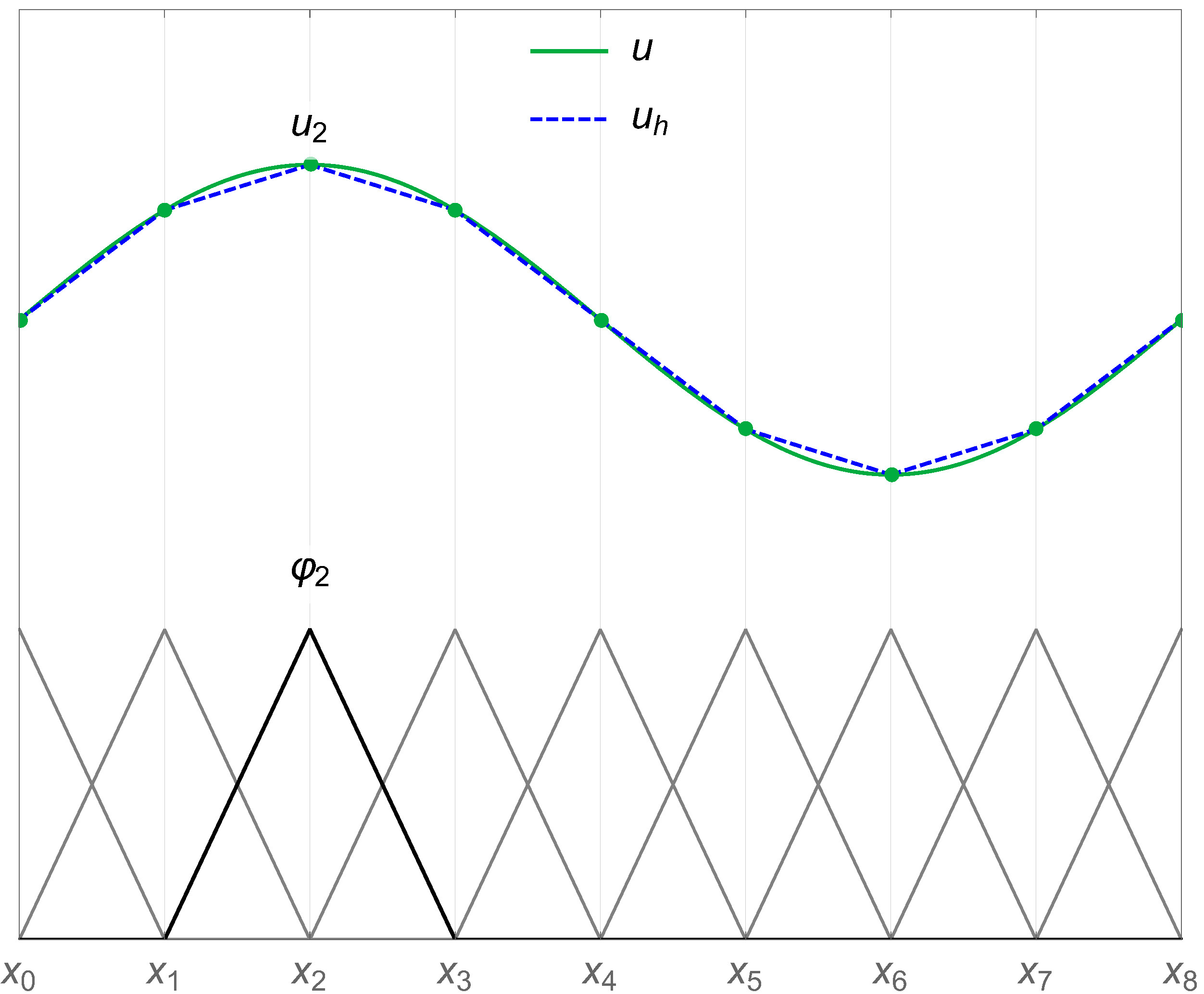
\begin{equation} \label {eq:nodal_basis_decomp} u_\text {h}\pqty {\vb {x}} = \sum _{i=1}^{N} u_\text {i} \varphi _\text {i}\pqty {\vb {x}} \end{equation}

\(N\) is the total number of nodes, and \(u_\text {i} = u_\text {h}(\vb {x}_\text {i})\) are the values assumed by the approximate solution at the nodes. Fig. 6.1 illustrates a possible approximation of the solution \(u\) through linear basis functions in a one-dimensional scenario. \(u\) could be taken to represent the electrical potential in a rod with non-uniform charge distribution. The rod is split into eight equal parts (which represent its triangulation), and the basis functions associated with each node have a value of one at their respective node, and 0 at all other nodes. It can be seen how \(u_\text {h}\), as defined by (6.48), can be used to approximate the continuous solution \(u\). One of the advantages of employing the finite element method is that it offers great freedom in the selection of discretization, both in the choice of elements and basis functions [130]. Moreover, it is possible to locally refine the mesh to obtain a better approximations in the regions where the solution varies quickly.

Determining the coefficients \(u_\text {i}\) gives a unique solution to the problem at hand. The values on \(\mathcal {N}_\text {D}\) are determined by the Dirichlet boundary conditions:

\begin{equation} \label {eq:dirichlet_discrete} u_\text {i} = u_\text {D}(\vb {x}_\text {i}) \qquad \forall \vb {x}_\text {i} \in \partial \Omega _\text {D} \end{equation}

All the remaining values can be determined by inserting \(u_\text {h}\) and \(v_\text {h}\) instead of \(u\) and \(v\) in (6.44), and then expressing both of them in terms of their nodal values through (6.48). Fulfilling (6.44) for the whole space \(V_\text {h}\) is equivalent to only considering the basis associated with the free nodes \(\Bqty {\varphi _\text {i} \, | \, \vb {x}_\text {i} \in \mathcal {N}_\text {f}}\), leading to the following expression:

\begin{equation} \label {eq:poisson_weak_discrete} \sum _{i} \Bqty {\int _{\Omega } \grad {\varphi _\text {i}} \vdot \grad {\varphi _\text {j}} \dd {\vb {x}}} \, u_\text {i} = \int _{\Omega } q \, \varphi _\text {j} \dd {\vb {x}} + \int _{\partial \Omega _\text {N}} g \, \varphi _\text {j} \dd {\vb {x}} \end{equation}

This equivalence needs to be valid for the whole set of basis functions associated with the free nodes. A matrix \(A \in \mathbb {R}^N\times \mathbb {R}^N\) for the right-hand side of (6.50) and a vector \(f \in \mathbb {R}^N\) for the left-hand side can be defined as

\begin{align} A_\text {ji} &= \int _{\Omega } \grad {\varphi _\text {i}} \vdot \grad {\varphi _\text {j}} \dd {\vb {x}} \, , \\ f_\text {j} &= \int _{\Omega } q \, \varphi _\text {j} \dd {\vb {x}} + \int _{\partial \Omega _\text {N}} g \, \varphi _\text {j} \dd {\vb {x}} \, . \end{align} Both \(A\) and \(f\) can be represented in terms of their components acting on the Dirichlet and free nodes:

\begin{equation} A = \begin{pmatrix} A_\text {DD} & A_\text {Df} \\ A_\text {fD} & A_\text {ff} \end {pmatrix}, \qquad f = \begin{pmatrix} f_\text {D} \\ f_\text {f} \end {pmatrix} \end{equation}

As only neighboring nodes have overlapping basis functions, \(A\) is a sparse matrix, with non-zero terms only around the diagonal. By considering the constraint (6.49), and the solution vector \(u = (u_\text {i}) \in \mathbb {R}^N\), \(u=\pqty {u_\text {D},u_\text {f}}^\text {T}\), (6.50) can be written as the following system of linear equations:

\begin{equation} \begin{pmatrix} I & 0 \\ A_\text {fD} & A_\text {ff} \end {pmatrix} \begin{pmatrix} u_\text {D} \\ u_\text {f} \end {pmatrix} = \begin{pmatrix} u_\text {D} \\ f_\text {f} \end {pmatrix} \end{equation}

\(I\) stands for the identity matrix. As the \(u_\text {D}\) values are known, the final symmetric system of \(N_\text {f}\) equations for the determination of the unknown \(u_\text {f}\) values is

\begin{equation} A_\text {ff}u_\text {f} = f_\text {f} - A_\text {fD}u_\text {D} \, . \end{equation}

6.2.2 Weak Formulation of the Micromagnetic Equations

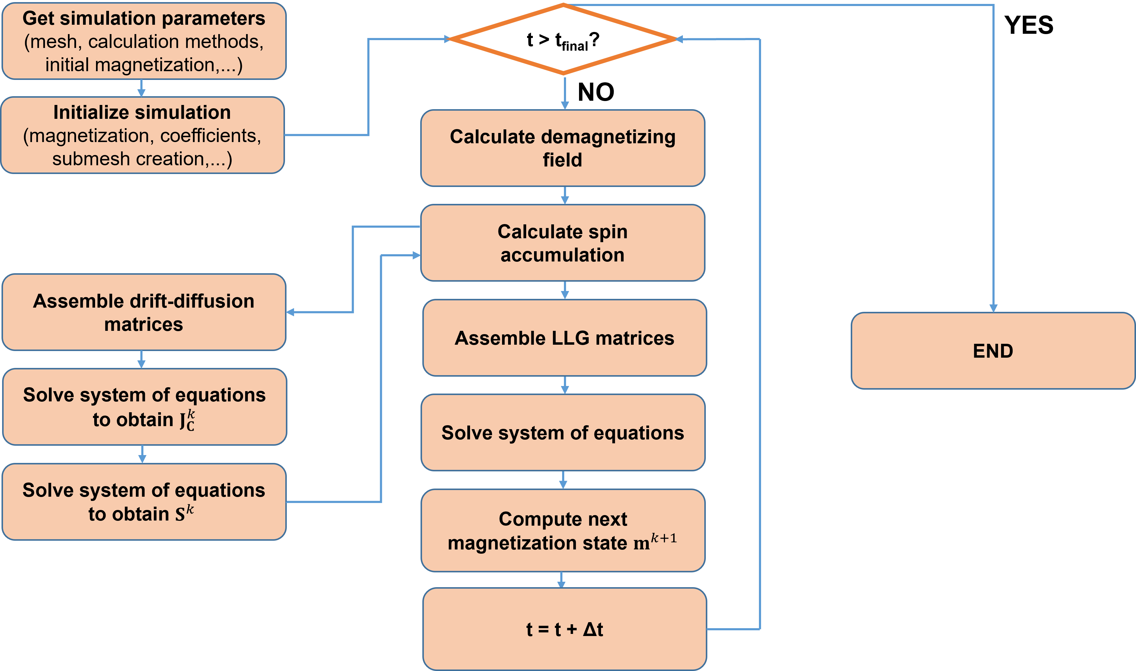
The implementation of a FE algorithm for the solution of the LLG equation has been of great interest for the solution of micromagnetic problems with meshes of varying complexity. First schemes for a numerical approximation of the weak LLG solution were proposed in [134], [135], by considering only the exchange field contribution to the effective field. In reference [136] the so-called tangent plane integrator scheme, solving for the discrete time derivative, was introduced, and was later generalized to include the full effective field [137], [138]. The unconditional convergence of the tangent plane integrator scheme and of the FE implementation of the spin and charge drift-diffusion equations was proven in [139], and later applied to metallic spin-valves in [23]. Here, the weak formulation of the tangent plane integrator and of the spin and charge transport equations, employed to obtain the results presented in these thesis, is reported. The flow-chart of the simulation process is presented in Fig. 6.2.

LLG Equation

The tangent plane scheme solves the LLG equation for the magnetization derivative \(\pdvline {\vb {m}}{t} = \vb {v}\). The weak formulation of the LLG equation comes from the expression

\begin{equation} \alpha \pdv {\vb {m}}{t} + \vb {m} \times \pdv {\vb {m}}{t}= \gamma _0 \, \vb {H}_\text {eff} - \gamma _0\pqty {\vb {m}\vdot \vb {H}_\text {eff}} \vb {m} \, , \label {eq:gilbert_for_weak} \end{equation}

which can be obtained by cross-multiplying (3.9) with \(\vb {m}\), and using the product rule \(\vb {a}\times \pqty {\vb {b}\times \vb {c}} = \pqty {\vb {c}\vdot \vb {a}}\vb {b} - \pqty {\vb {a}\vdot \vb {b}}\vb {c}\) together with the constraint \(\abs {\vb {m}} = 1\). For the FE implementation, the magnetization is taken to be a piecewise affine, globally continuous function [83]. Each component belongs to the Sobolev space \(H^1\). It is the space of functions in \(L^2\) that additionally admit a weak gradient which also belongs to \(L^2\) [138]. The weak gradient is a generalization of the gradient, defined with the help of the test functions and valid in an integral sense, and its existence is needed to be able to evaluate terms containing spatial derivatives in the weak formulation. The notation for the vector space of the magnetization is \(\vb {H}^1\). Instead of looking for the solution \(\vb {v}\) in the same space of the magnetization, the solution space \(V_\text {T}\) is restricted to vectors tangent to the magnetization, so that \(V_\text {T} = \Bqty {\bm {w} \in \vb {H}^1 \, | \, \vb {m}\vdot \bm {w} = 0}\). The test functions are also restricted to the same space, so that the weak formulation of (6.55) results in

\begin{gather} \int _{\omega } \pqty {\alpha \vb {v} + \vb {m} \times \vb {v}} \vdot \bm {w} \dd {\vb {x}} = \gamma _0 \, \int _{\omega } \vb {H}_\text {eff}(\vb {m}) \vdot \bm {w} \dd {\vb {x}} \, , \label {eq:llg_weak_small} \end{gather} where \(\omega \) is the subdomain containing only the magnetic parts of the structure under analysis. The last term on the right-hand side of (6.55) is not present, as the test functions are restricted to the tangent space \(V_\text {T}\). The time derivative \(\vb {v}\) at a certain time \(t^\text {k}\) is obtained by setting [83]

\begin{equation} \vb {m}^\text {k+1} = \vb {m}^\text {k} + \theta \delta t \vb {v} \, , \label {eq:mag_theta} \end{equation}

where \(\delta t\) is the time-step, and \(\theta \) is a parameter between 0 and 1, with the value 0 leading to a fully explicit scheme and 1 to a fully implicit one. Each effective field contribution can be treated with a different value of \(\theta \). In the implementation employed for this work, \(\theta \) is different from 0 only for the exchange field contribution (3.17), where the value 1 is employed for stability reasons [140]. The weak formulation employed for the computation of the magnetization dynamics by the FE solver, with the inclusion of the torque terms coming from (6.1), is then

\begin{gather} \nonumber {\int _\omega \pqty {\alpha \vb {v} + \vb {m}^\text {k} \times \vb {v}} \vdot \bm {w} \dd {\vb {x}} + \frac {2A \gamma }{M_S} \delta t \int _\omega \grad {\vb {v}} : \grad {\bm {w}} \dd {x} = } \\ \nonumber {- \frac {2 A \gamma }{M_S} \int _\omega \grad {\vb {m}^\text {k}} : \grad {\bm {w}} \dd {\vb {x}} + \gamma _0 \int _\omega \pqty {\vb {H}_\text {ext}+\vb {H}_\text {ani}(\vb {m}^\text {k})+\vb {H}_\text {demag}(\vb {m}^\text {k})} \vdot \bm {w} \dd {x} + } \\ {+ \frac {D_\text {e}}{M_\text {S}} \int _\omega \pqty {\frac {\vb {S}^\text {k}}{\lambda _J^2} + \frac {\vb {m}^\text {k}\times \vb {S}^\text {k}}{\lambda _\varphi ^2}} \vdot \bm {w} \dd {\vb {x}}} \, , \label {eq:llg_weak_formulation} \\ \vb {m}^\text {k+1}=\frac {\vb {m}^\text {k} + \delta t \, \vb {v}}{\abs {\mathbf {m}^\text {k} + \delta t \, \vb {v}}} \, . \label {eq:llg_time_update} \end{gather} The right-hand side of (6.58b) is evaluated nodewise, \(\omega \) indicates the magnetic subdomains, and \(\grad {\vb {a}} : \grad {\vb {b}} = \sum _\text {ij}\pqty {\partial a_\text {i} / \partial x_\text {j}}\pqty {\partial b_\text {i} / \partial x_\text {j}}\) is the Frobenius inner product of two matrices. The exchange field contribution (3.17), together with (6.57), gives rise to the second term on the left-hand side and to the first term on the right-hand side. The boundary integrals arising from the weak formulation of this contribution are put to zero by the Neumann boundary condition (3.41), applied on the external boundary of the magnetic region \(\partial \omega \). The equations are subject to the initial condition \(\vb {m}(0) = \vb {m}^0\). The system of equations resulting from the FE implementation of this weak formulation includes the tangent plane constraint \(\vb {m}\vdot \bm {w} = 0\), and the solution at each time-step is computed through a solver based on the generalized minimal residual (GMRES) method, provided by the library MFEM. The GMRES method is an iterative algorithm for the numerical solution of an indefinite nonsymmetric system of linear equations, as is the case of FE implementation of (6.58a) due to the presence of the cross-product terms. Material parameters that can differ from subdomain to subdomain are treated as piecewise constant functions, unless differently stated. The contribution of the demagnetizing field \(\vb {H}_\text {demag}\) is evaluated only on the disconnected magnetic domain by using a hybrid approach combining the boundary element method and the FE method [141], [142].

Spin and Charge Drift-Diffusion Equations

The weak formulation for the computation of the spin accumulation is derived from (6.38). The equations are solved for the magnetization \(\vb {m}^\text {k}\) at each time-step, and the resulting spin accumulation \(\vb {S}^\text {k}\) is employed in (6.58a).

For the computation of the charge potential and current, a Laplace equation is solved for the whole domain \(\Omega \), with the weak formulation

\begin{gather} \int _{\Omega } \sigma \grad {V} \vdot \grad {v} \dd {\vb {x}} = 0 \, ,\\ \int _{\Omega } \vb {J}_\text {C} \vdot \bm {v} \dd {\vb {x}} = -\int _\Omega \sigma \grad {V} \vdot \bm {v} \dd {\vb {x}} \, , \label {eq:cc_weak_proj} \end{gather} where \(v\) represents a test function belonging to \(H^1\), while \(\bm {v}\) is a test function in \(\vb {H}^1\). \(V\) belongs to \(H^1\), and equation (6.59b) is employed to obtain a projection of \(\vb {J}_\text {C}\) in the \(\vb {H}^1\) function space [83]. Dirichlet conditions are applied to prescribe the voltage at the contacts. The Neumann condition \(\sigma \grad {V}\vdot \vb {n} = 0\) is assumed on external boundaries not containing an electrode. Special treatment of the conductivity \(\sigma \) results in an implementation capable of reproducing the charge current dependence on the TMR and relative direction of the magnetization vectors in the FL and RL of an MTJ, as will be shown in Chapter 7. The solution of the system of equations resulting from the FE implementation of (6.59) is computed through a solver based on the conjugate gradient (CG) method, provided by the library MFEM. The CG method is an algorithm for the numerical solution of systems of linear equations whose matrix is positive-definite, as is the case of the FE implementation of (6.59).

The weak formulation of the spin drift-diffusion equations presented in [23] is generalized to apply to (6.38), which includes the additional spin dephasing term, resulting in the following expression:

\begin{gather} \nonumber {D_\text {e} \int _{\Omega } \pqty {\grad {\vb {S}} - \beta _\sigma \beta _\text {D} \vb {m} \otimes \pqty {\pqty {\grad {\vb {S}}}^\text {T} \mathbf {m}}} : \grad {\bm {v}} \dd {\vb {x}} + } \\ \nonumber {+ D_\text {e} \int _{\Omega } \pqty {\frac {\vb {S}}{\lambda _{sf}^2} + \frac {\vb {S} \times \vb {m}}{\lambda _{J}^2} + \frac {\vb {m} \times \pqty {\vb {S} \times \vb {m}}}{\lambda _{\varphi }^2}} \vdot \bm {v} \dd {\vb {x}} = } \\ \frac {\mu _B}{e} \beta _\sigma \int _{\omega } \pqty {\vb {m} \otimes \vb {J}_\text {C}} : \grad {\bm {v}} \dd {\vb {x}} - \frac {\mu _B}{e} \beta _\sigma \int _{\partial \Omega \cap \partial \omega } \pqty {\pqty {\vb {m} \otimes \vb {J}_\text {C}}\vb {n}} \vdot \bm {v} \dd {\vb {x}} \label {eq:spin_weak_form} \end{gather} \(\bm {v}\) represents again a test function belonging to \(\vb {H}^1\), \(\vb {S}\) also belongs to \(\vb {H}^1\), and \(\partial \Omega \cap \partial \omega \) indicates the shared external boundary of the whole domain \(\Omega \) and magnetic subdomain \(\omega \). The boundary integrals arising from the weak formulation are put to zero by the Neumann condition \(\pqty {\grad {\vb {S}}}\vb {n} = \vb {0}\), assumed on external boundaries. For contacting regions longer than the spin-flip length, this condition is equivalent to an exponential decay of \(\vb {S}\) towards the electrodes [23], [25]. The charge current \(\vb {J}_\text {C}\) is the one computed from (6.59). The solution of the system of equations resulting from the FE implementation of (6.60) is computed through a solver based on the GMRES method, provided by the library MFEM, as due to the cross product terms the FE implementation of (6.60) results in a nonsymmetric system of linear equations.