Computation of Torques
in Magnetic Tunnel Junctions

Chapter 7 Charge Current Redistribution and MTJ Torque Magnitude in the Finite Element Drift-Diffusion Formalism

This chapter focuses first on the development of an approach for reproducing the charge current density dependence on the TMR and on the local angle between magnetization vectors of an MTJ in a FE setting. Then, the dependence of the torque on the various parameters entering the spin and charge drift-diffusion equations is analyzed, and it is shown how such parameters can be tuned to reproduce the torque magnitude expected in MTJs by the Slonczewski expression. The results hereby presented were published by the author in references [143],[144], [145], [146], [147], and [148]. All the reported FE solutions are computed in meshes composed of tetrahedral elements.

7.1 Reproduction of the TMR Effect

MTJs present a strong resistance dependence on the relative magnetization orientation in the FL and the RL, mainly determined by the polarized tunneling process. The dependence of the conductance on the angle between magnetization vectors can be expressed as [16], [64], [65], [99]

\begin{equation} \label {eq:TMR_conductance_pol} G\pqty {\theta } = G_0 \pqty {1+P_\text {RL}P_\text {FL}\cos \theta } \, , \end{equation}

where \(G_0=\pqty {G_\text {P}+G_\text {AP}}/{2}\), and \(\theta \) is the angle between the unit magnetization vector in the RL \(\vb {m}_\text {RL}\) and in the FL \(\vb {m}_\text {FL}\), \(\cos \theta =\vb {m}_\text {RL}\vdot \vb {m}_\text {FL}\). This expression is equivalent to (2.4) when taking Julliere’s expression (3.51) into account.

In Chapter 4, an analytical solution for the charge current density in an MTJ was reported, which was able to reproduce the voltage drop at the barrier and the current density dependence on the TMR value and on the local angle between the magnetization vectors. This, however, required to solve the Laplace equation separately in the two FM layers. The approach needs to be adapted to a FE implementation, with the solution computed simultaneously in the whole MTJ structure. In order to reproduce both the TMR effect and the angular dependence of the resistance, the oxide layer is modeled as a poor conductor, whose low conductivity depends on the relative magnetization vectors orientation as

\begin{equation} \label {eq:conductivity_FEM} \sigma \pqty {\vb {m}_\text {RL},\,\vb {m}_\text {FL}} = \sigma _0 \pqty {1+ P_\text {FL}\,P_\text {RL}\vb {m}_\text {RL}\vdot \vb {m}_\text {FL}} \, , \end{equation}

where \(\sigma _0=G_0\,d_\text {TB}/S\) is the conductivity of the tunnel barrier, with \(d_\text {TB}\) and \(S\) the thickness and surface area of the tunnel barrier, respectively. While the expression for \(\sigma _0\) depends linearly on \(d_\text {TB}\), the average conductance of the TB \(G_0\) decays exponentially with the barrier thickness. \(\vb {m}_\text {RL(FL)}\) is the magnetization of the RL(FL) close to the interface. It is a manifestation of Ohm’s law relating the voltage and the charge current through a structure with many transversal modes [123], [127].

A solution for the electric potential and current density in an FE setting can be computed through equation (6.59). The conductivity is described by a piecewise constant coefficient in the metallic layers, and by a coefficient based on equation (7.2) in the tunneling layers. In the scope of the MFEM library [149], only the data associated with a local element can be accessed during the assembly of the system matrices, while the computation of (7.2) in the TB requires knowledge of the magnetization vectors in the neighboring FM layers. In order to get access to the magnetization values, the coefficient describing the TB conductivity is initialized as follows:

• • For each point inside the TB where the conductivity needs to be computed, referred to as integration point, the solver loops through the integration points of the RL and FL elements closer to the interfaces

• • The RL and FL points near to or at the interface with coordinates closest to the TB point are selected

• • The integration point number and element number associated with the nearest RL and FL points are mapped to the coordinates of the TB points

In a transient simulation, the search is carried out only during the initialization of the solver. At every time-step, the data necessary for the computation of (7.2) can be accessed through the generated maps, without the need to repeat the search procedure and waste computational time.

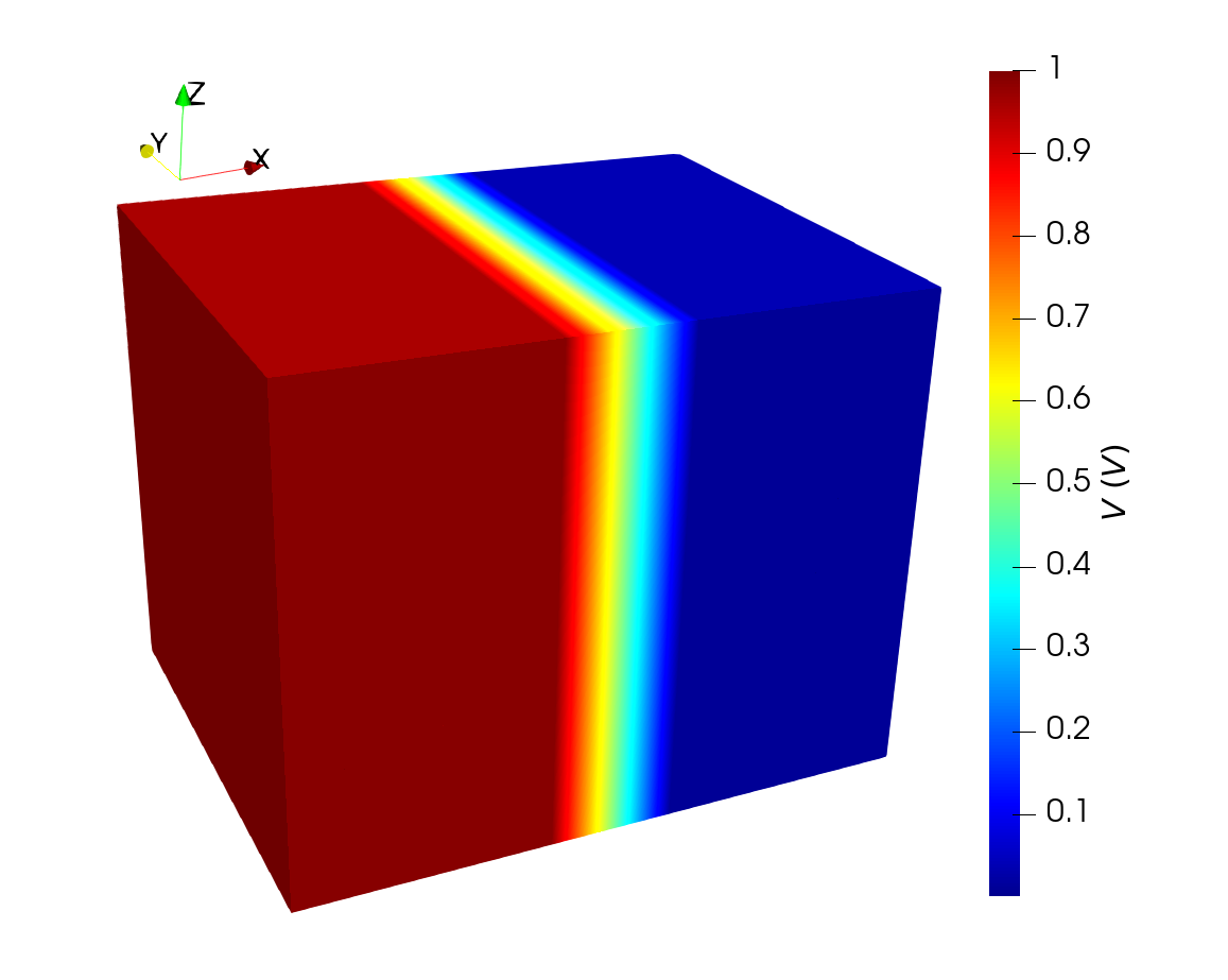
The FE solution obtained from equations (6.59) and (7.2) is first computed in a mesh reproducing the structure schematized in Fig. 4.1. The lateral dimensions are 10\(\times \)10 nm\(^2\). The mesh was prepared by modifying one of the built-in MFEM meshes. The magnetization distribution is taken to be parallel in the center of the structure, and anti-parallel on the sides. The potential is fixed with Dirichlet conditions on the left and right boundaries. The values of conductivity, resistance and bias voltage are the same as the ones employed for the analytical solution presented in Chapter 4. The voltage and x-component of the current density computed via the FE method are reported in Fig. 7.1. The distribution of the latter is evidenced on planes located at the contacts and at the TB interfaces. Both the voltage drop localized at the TB and the TMR dependent redistribution of \(\vb {J}_\text {C}\) are reproduced, in agreement with the analytical results. The current density flow is higher in the center of the structure, where the parallel magnetization vectors favor the tunneling process and grant a better conductance.

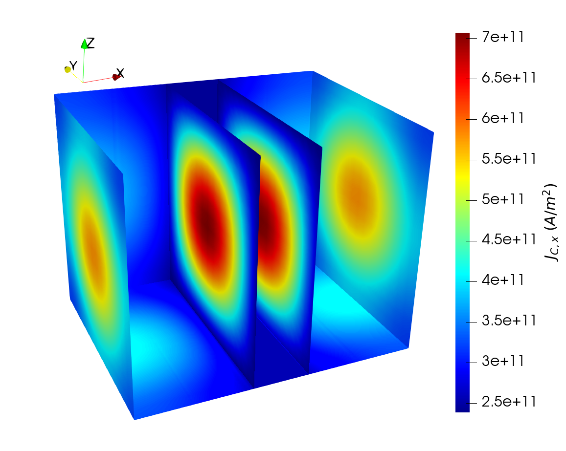
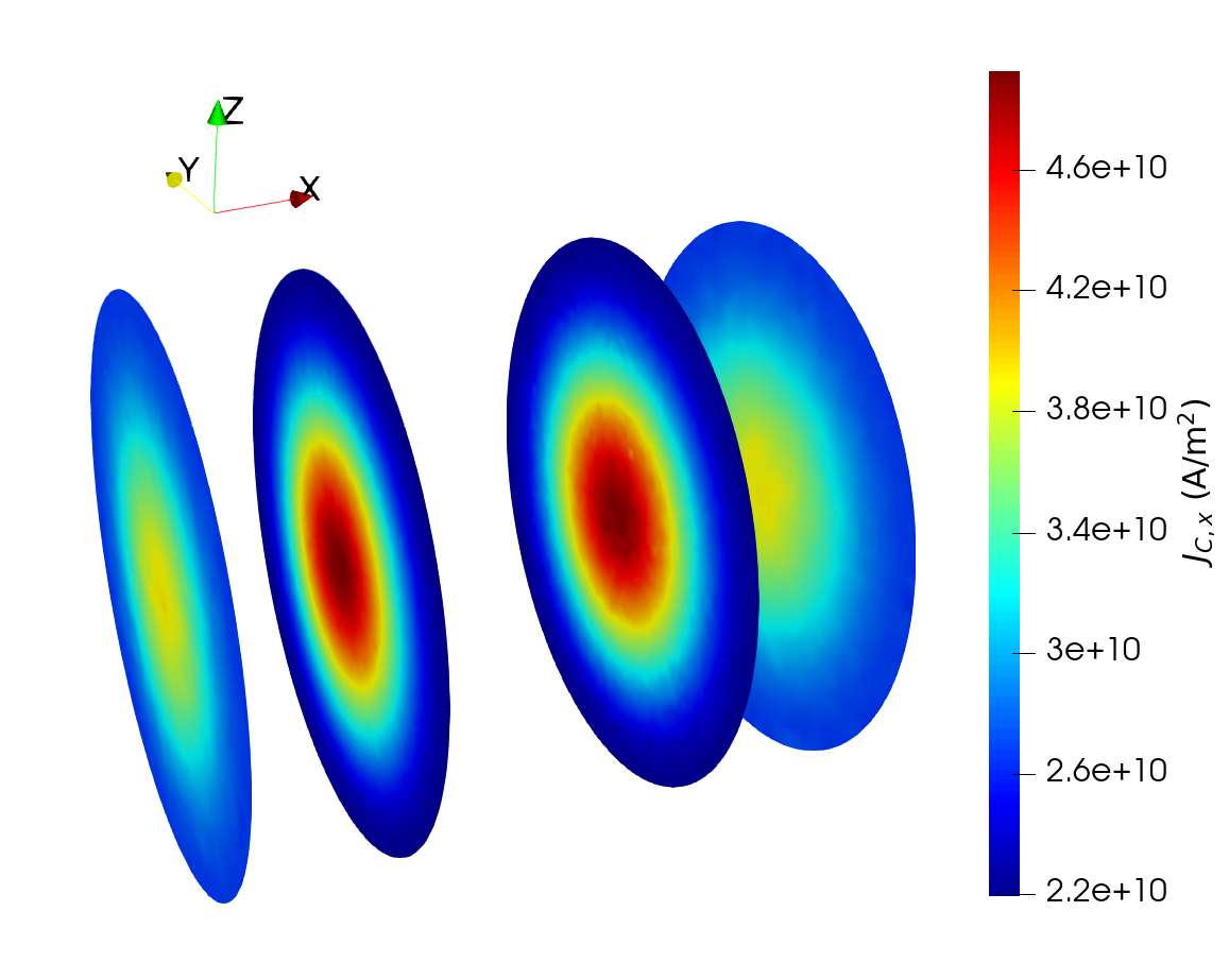
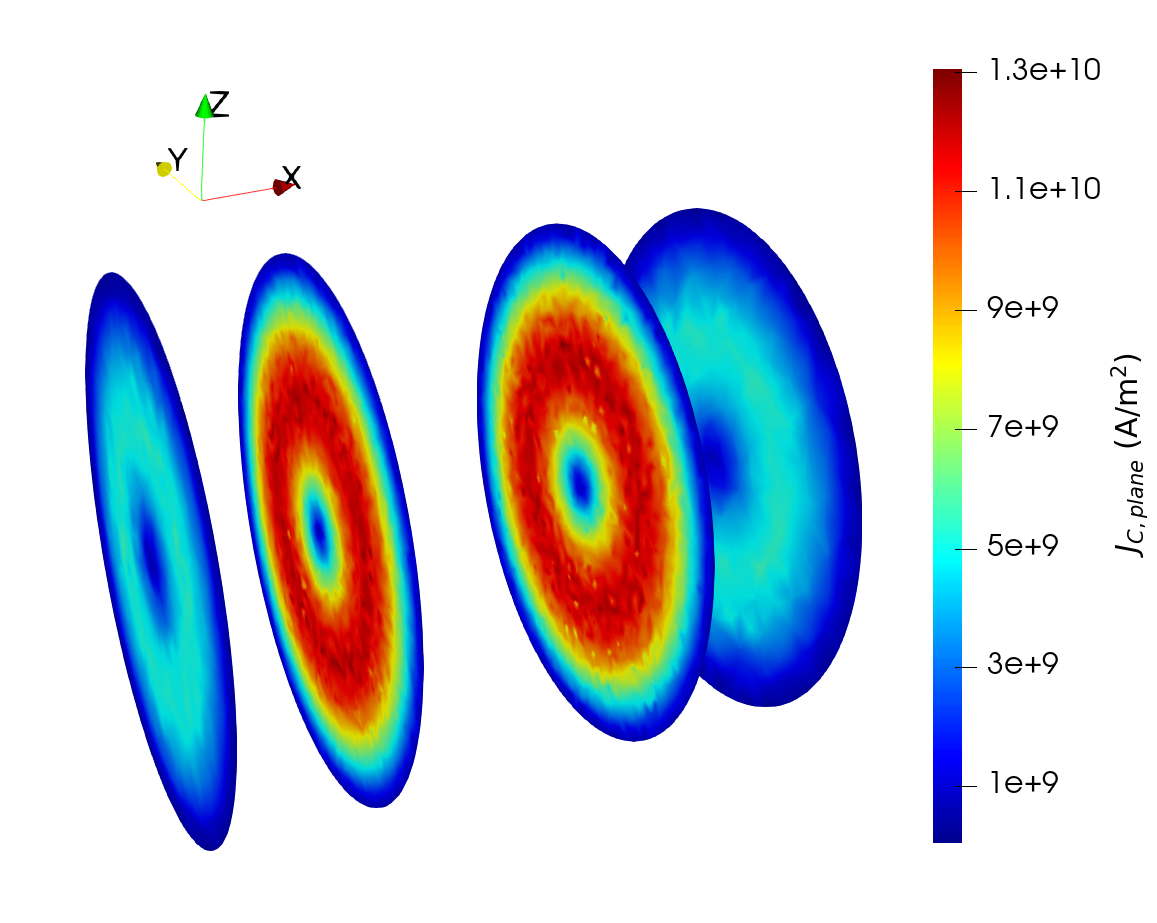
Thanks to the FE implementation, it is then possible to run the solver on meshes representing more realistic MTJ structures. As an example, the current density distribution is computed for the structure reported in Fig. 1.1. This mesh presents a circular cross-section, and includes 50 nm long nonmagnetic contacts. The mesh was prepared by employing the open-source software Netgen, part of the NGSolve package [150]. Dirichlet conditions are employed to apply the bias voltage on the left contact and fix the voltage value on the right one to 0. The cylindrical stack has a diameter of 40 nm, RL and FL of 2 nm thickness, and TB of 1 nm thickness. The conductivity of the nonmagnetic layers is \(\sigma _\text {NM}=5\times 10^{6}\) S/m. The values of conductivity in the FM layers, TB average conductance and applied bias voltage are \(\sigma _\text {RL}=\sigma _\text {FL}=10^{6}\) S/m, \(G_0=4.76 \times 10^{-5}\) S, and \(V_0=1\) V, respectively, and the magnetization configuration is the same as the one employed for Fig. 7.1. The obtained TMR- and magnetization-dependent current density distribution is reported in Fig. 7.2. Here, all the cross-sections are located inside the nonmagnetic regions. The inner ones are close to the interface between the FM and NM layers, while the outer ones are further inside the nonmagnetic contacts. Fig. 7.2(a) shows how the current density’s x-component is non-uniform also inside of the nonmagnetic regions. Due to conservation of the current flow, the current density is redistributed in the yz-plane of the metallic layers. This is evidenced by Fig. 7.2(b), where the modulus of its in-plane components, \(J_\text {C,plane}=\sqrt {J_\text {C,y}^2+J_\text {C,z}^2}\), is reported.

7.2 Finite Element Solution for the Spin Accumulation

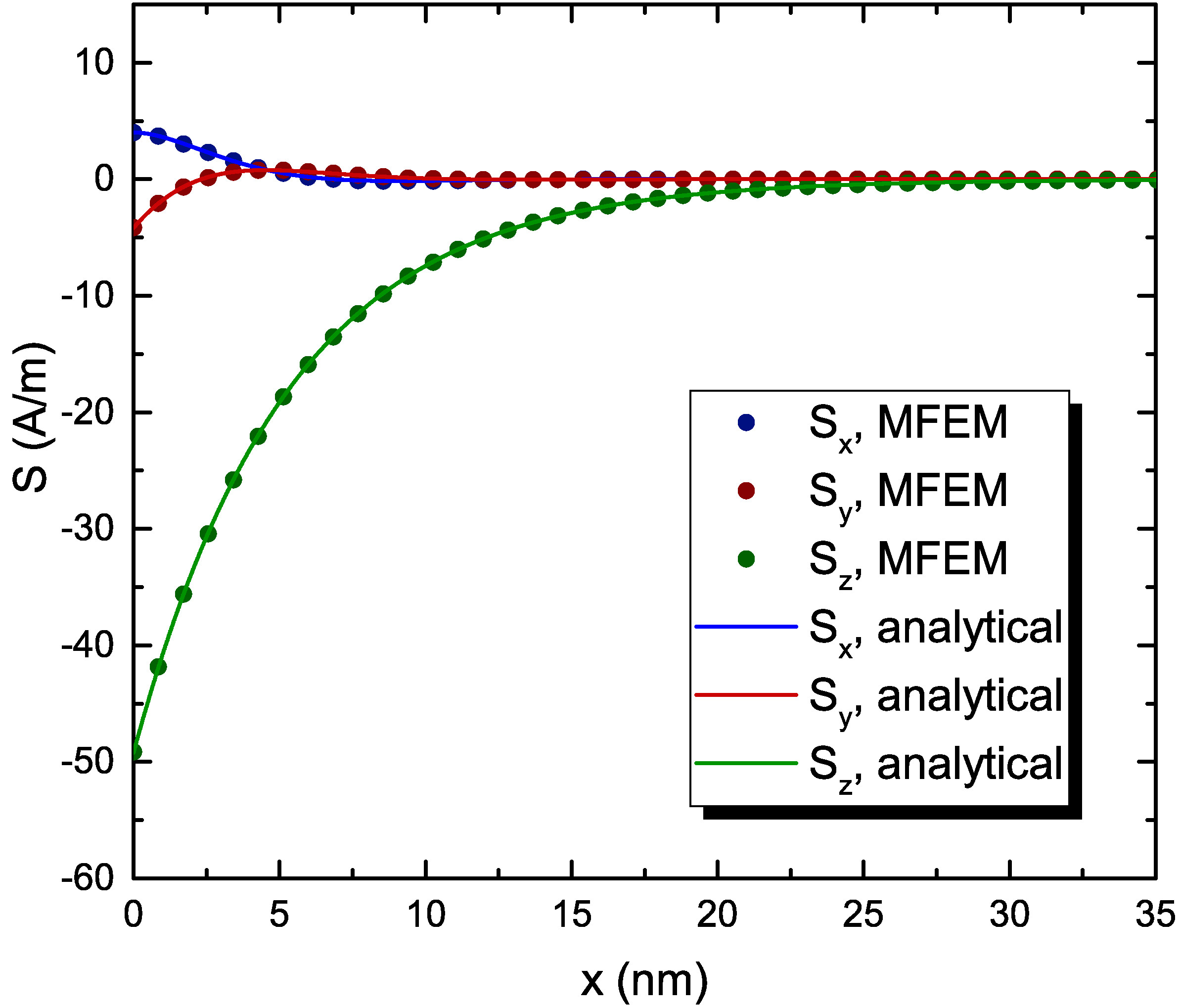
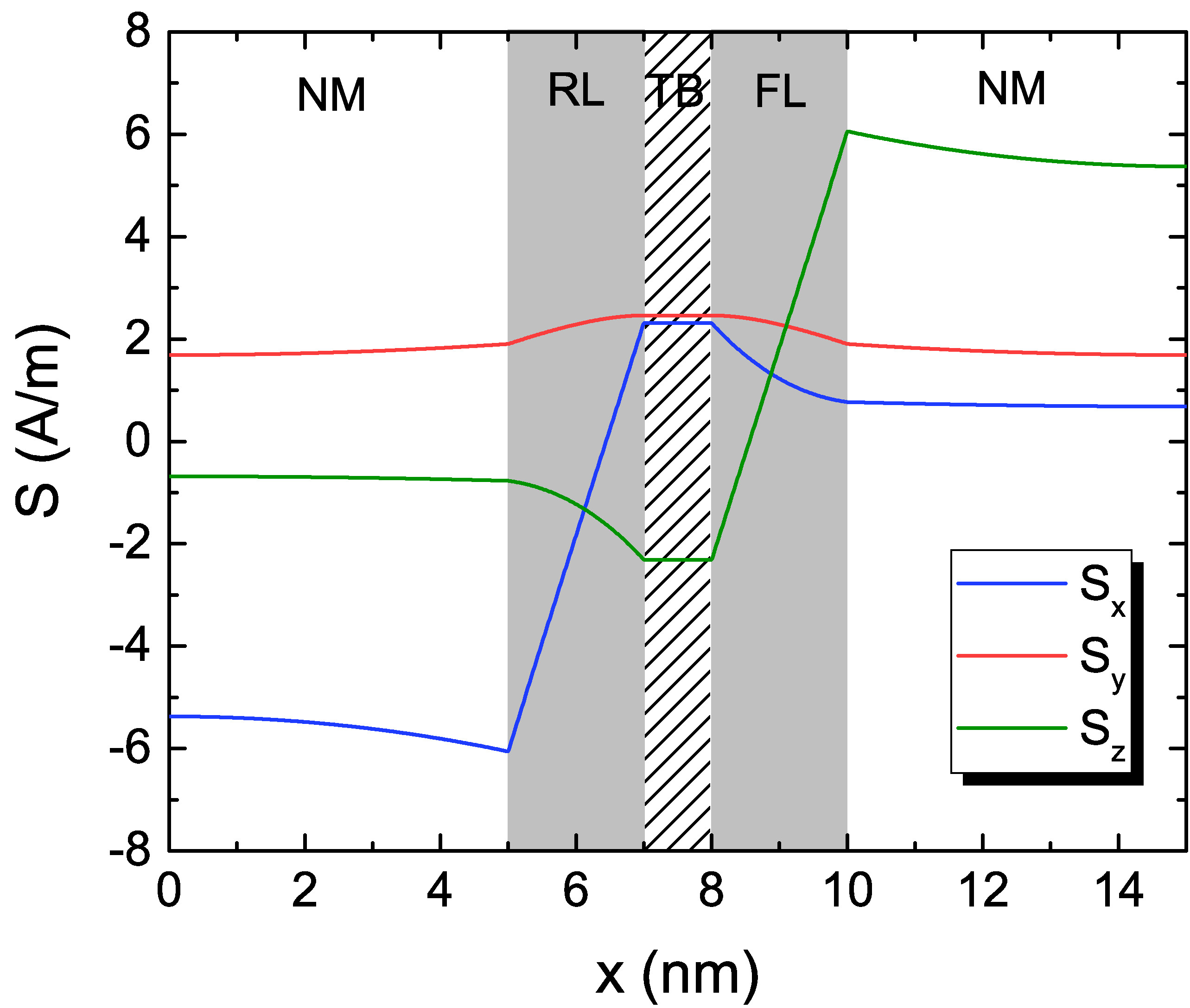
The MFEM implementation of the weak formulation (6.60), which allows to obtain a solution for the spin accumulation in a FE setting, is first tested against known analytical results [98]. The parameters employed for these simulations, taken from [23] and [25], are reported in Table 7.1. The spin accumulation and spin torques are computed for the FL of a metallic spin-valve, magnetized along the z-direction, with a fully spin-polarized current coming from the left boundary, at x=0 nm. Such a current could be generated by a half metallic thick RL [98]. The magnetization in the RL is chosen to point in the negative y-direction. For this simulation, the term containing \(\lambda _{\varphi }\) is not considered, and a fixed current density flowing in the negative x-direction, with value \(J_\text {C,x}=-10^{11}\) A/m\(^2\), is applied. The layer is taken to be 60 nm long. As the magnetization is uniform, the lateral dimensions of the structure do not have any impact on the solution. The layer’s mesh was generated by using Netgen. In Fig. 7.3 the analytical result for the spin accumulation is compared to the one computed by employing the MFEM solver, showing an excellent agreement between the two.

The torque acting on the magnetization is related to the spin current via (6.13), where the term describing spin-flip relaxation is subtracted from the divergence of the spin current. In case of negligible spin-flip scattering, the relation becomes

\begin{equation} \vb {T}_\text {S}=-\div {\tilde {\vb {J}}_\text {S}} \, . \label {eq:sc_div} \end{equation}

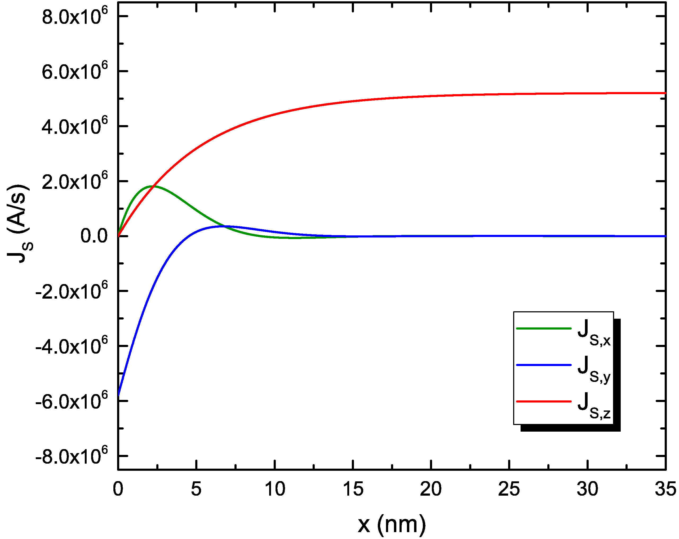
Equations (6.13) and (7.3) should give compatible values for the torque, provided that \(\lambda _\text {J}\) is shorter than \(\lambda _\text {sf}\). This is usually the case for most ferromagnetic materials [98], [151]. In order to check the validity of these assumptions, the torque obtained from both expressions is compared. First, the spin current flowing in the x-direction, \(\vb {J}_\text {S,x}\), is computed from the spin accumulation solution of Fig. 7.3 using (6.6), and is reported in Fig. 7.4(a). It can be noted, that near the interface the spin current is fully polarized along the direction of the magnetization in the RL. The component parallel to the RL magnetization is quickly absorbed. Precession of the spin current around the FL magnetization direction creates a component in the x-direction, perpendicular to the common plane of the magnetization vectors in the RL and the FL. This component is also absorbed on the length scale dictated by \(\lambda _J\). The spin current gets then polarized in the direction of the magnetization in the FL.

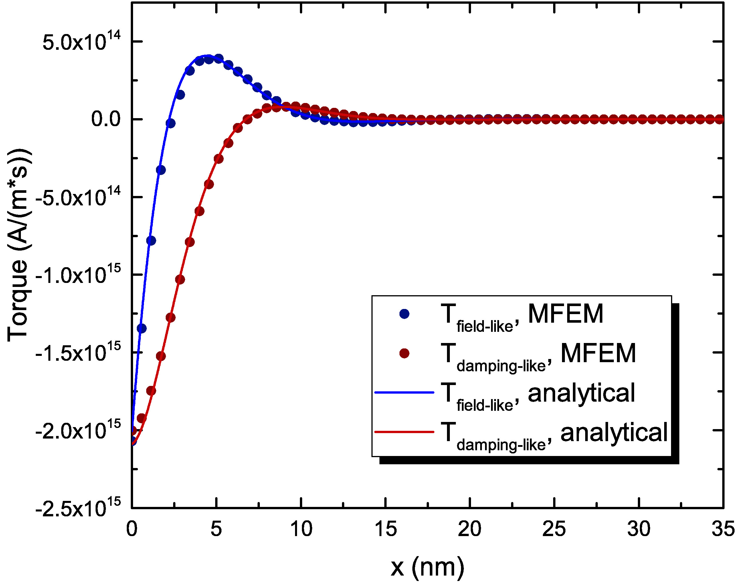
The comparison of the torques computed using (6.13) and (7.3) is reported in Fig. 7.4(b), where the former is labeled as \(\vb {T}_1\), while the latter is labeled as \(\vb {T}_2\). The damping-like component of the torque, also called adiabatic component, is the one lying in the plane formed by the magnetization vectors in the RL and the FL, and tends to align them in the parallel or anti-parallel configuration, depending on the sign of the electric current. It acts along the same axis as the Gilbert damping term in the LLG equation. With \(\vb {m}\) the unit magnetization vector in the layer where the torque is computed and \(\vb {p}\) the one in the polarizing layer, this torque component lies in the direction defined by \(\vb {m}\times \pqty {\vb {m}\times \vb {p}}\). In the present simulation, it lies along the y-axis. The field-like component, also referred to as non-adiabatic component, is perpendicular to the plane, and creates a precessing motion, in a manner analogues to an external field. This component lies along the direction defined by \(\vb {m}\times \vb {p}\). Here, it lies along the x-axis. Both components of the torque computed using the two expressions are in very good agreement, so that the use of (7.3) for computing the torques directly from the spin current is justified if \(\lambda _{J}\),\(\lambda _{\varphi } < \lambda _{sf}\).

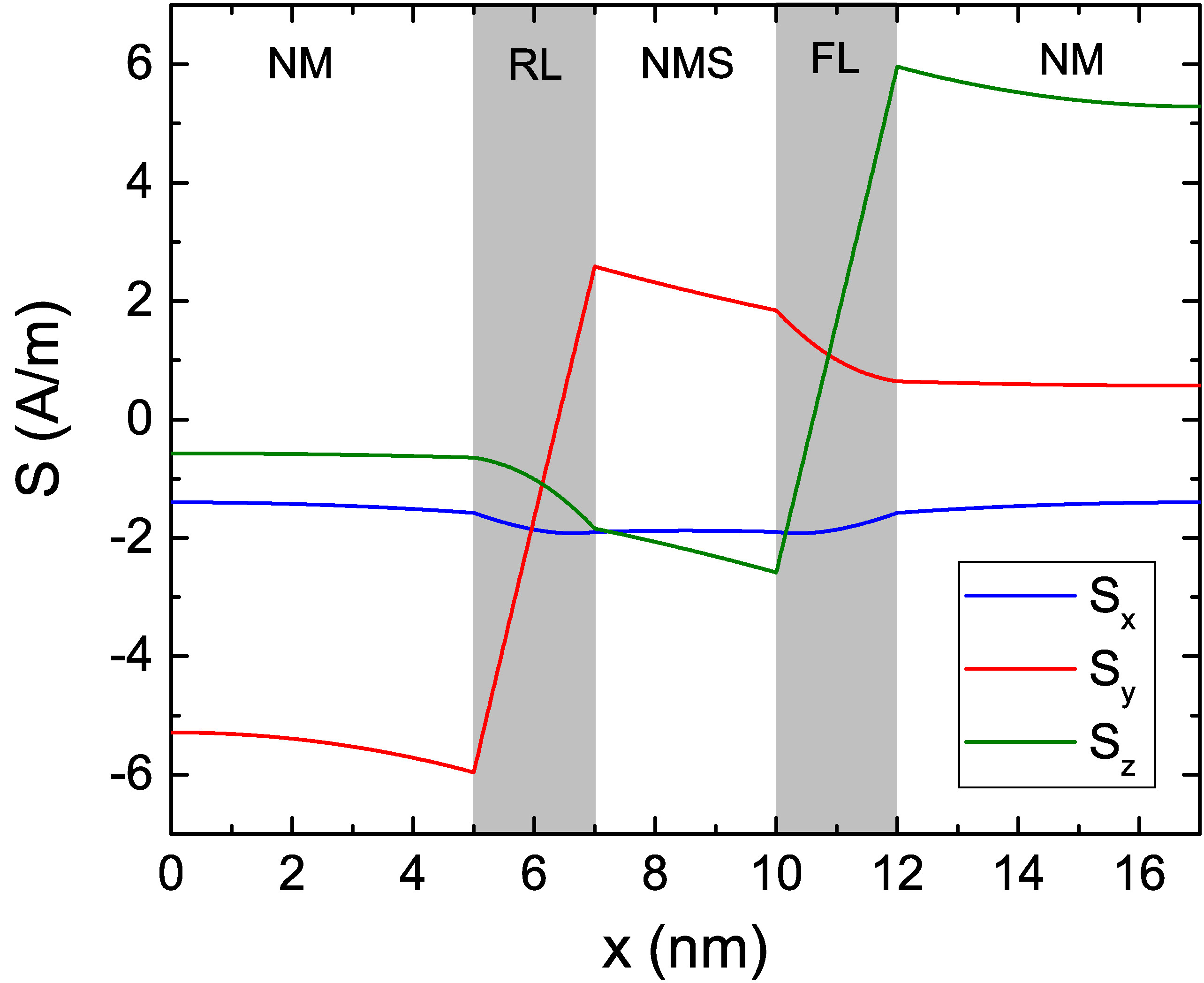
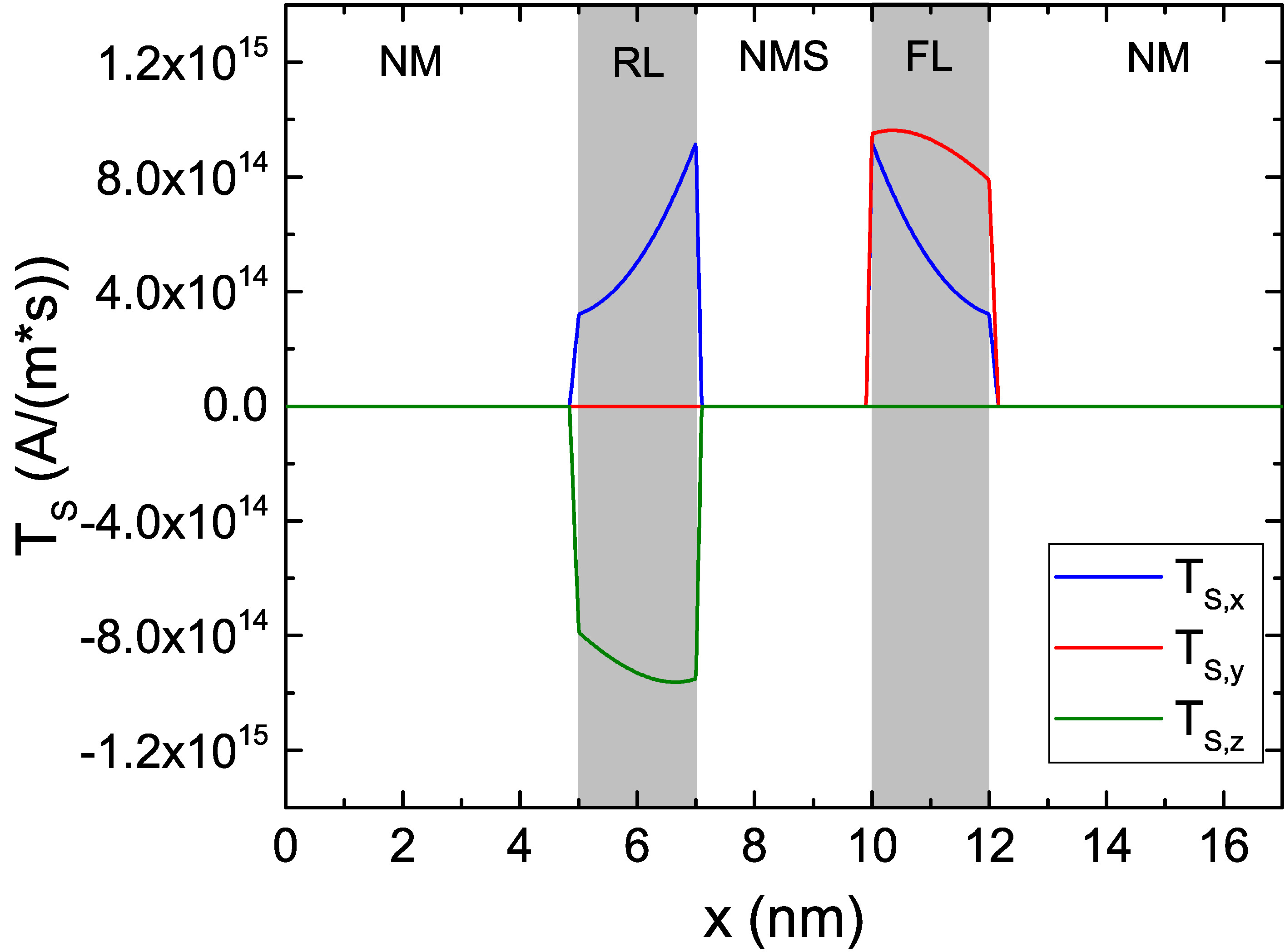
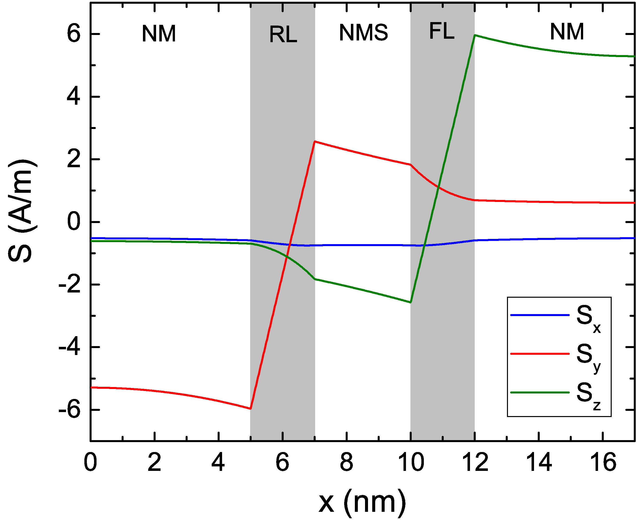
After verifying the accuracy of the FE implementation in computing the spin accumulation and torques, the formalism can be applied to multi-layered structures, in order to obtain the magnetization dynamics in STT-MRAM cells, composed of multiple magnetic and nonmagnetic layers. To further test the MFEM implementation, the software is employed to compute the spin accumulation in the same scenario as reported by Abert et al. in [23]. The structure under study is a spin valve with 5 nm NM contacts, 2 nm FM layers, and a 3 nm nonmagnetic spacer (NMS). The structure is magnetized in-plane, with the magnetization in the RL pointing towards the y-direction and the one in the FL pointing towards the z-direction. A uniform current density flows through the structure in the x-direction, with value \(J_\text {C,x}=-10^{11}\) A/m\(^2\). The employed parameters are the ones reported in Table 7.1, without the spin dephasing term. The obtained spin accumulation is reported in Fig. 7.5(a), showing a good agreement with the results by Abert et al..

By looking at (6.38) it can be noted, that the source of the spin accumulation comes from spatial variations of the magnetization. In the present simulation, the magnetization is homogeneous within the FM layers, and the only variation happens at the interfaces with the NM layers, where all the magnetization components go abruptly to zero. The spin accumulation is thus generated at such interfaces, and then diffuses inside the layers. With this set of parameters, the spin accumulation components transverse to the magnetization direction are not completely absorbed inside the FM layers, as they are too thin. This can also be observed in the resulting torque, computed from (6.13) and reported in Fig. 7.5(b). Both a damping-like component (along y in the FL) and a field-like component (along z in the FL) are present, and do not completely decay inside the FM layers.

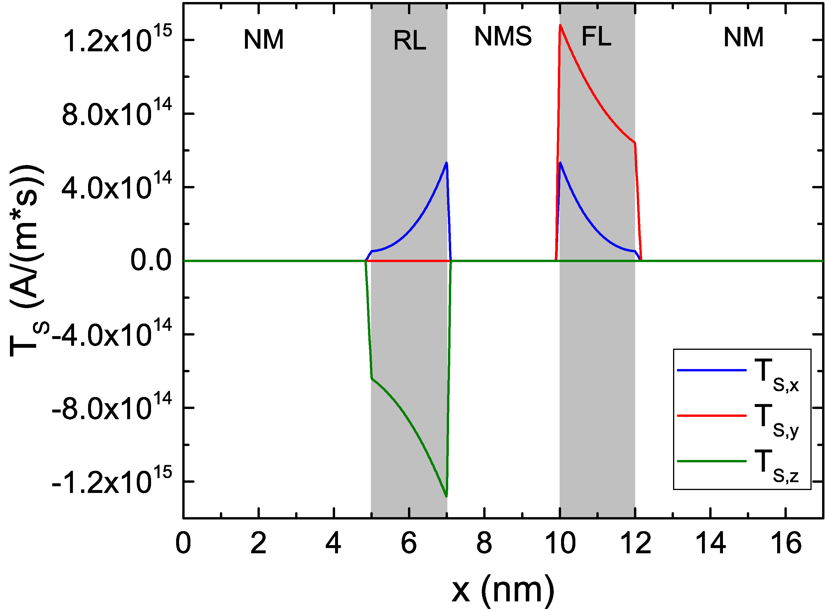
The shape of both the spin accumulation and torque is modified by the inclusion of the spin-dephasing term, especially when \(\lambda _\varphi \simeq \lambda _{J}\). The spin accumulation and torque computed by using \(\lambda _{\varphi } = \lambda _{J}\), with the torque obtained through (6.1), are reported in Fig. Fig. 7.5(c) and Fig. 7.5(d), respectively. The presence of the spin-dephasing term both enhances the torque absorption and modifies the relative values of the damping-like and field-like components, so that its inclusion can more accurately capture the interaction between magnetization and spin accumulation.

7.3 Torque Evaluation in Spin-Valve Structures

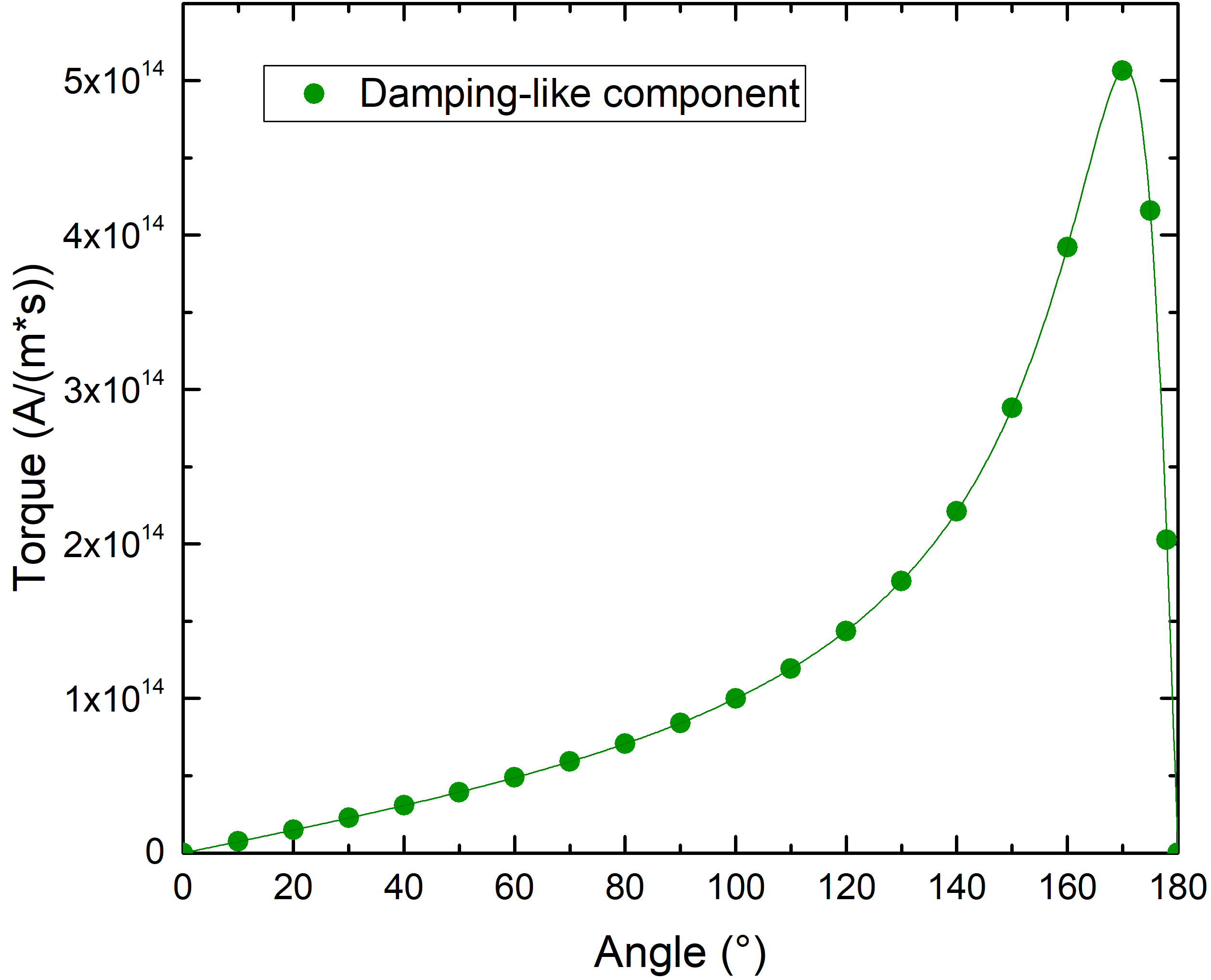
The possibility to compute the spin accumulation in a spin-valve structure gives the opportunity to compare the angular dependence of the damping-like torque obtained from the drift-diffusion implementation with the one obtained from the Slonczewski expression (3.48), which was derived by considering only ballistic transport in a symmetric stack [14]. The simulations are run in the same spin-valve structure described before, with a thinner 1 nm spacer layer to reduce the spin accumulation decay between the FM layers. The spin-flip length in the NM leads, \(\lambda _\text {sf}\), is set to 100 nm, while the remaining parameters are the ones reported in Table 5.1, including the dephasing length \(\lambda _{\varphi }\). The average torque acting on the FL is computed as

\begin{equation} \label {eq:avg_fl_torque} \vb {T}_\text {S,FL}=\frac {1}{d_\text {FL}}\int _{x_\text {FL}}^{x_\text {FL}+d_\text {FL}} \vb {T}_\text {S} dx \, , \end{equation}

where \(x_\text {FL}\) is the x-coordinate of the interface between middle layer and FL, and \(d_\text {FL}\) is the thickness of the FL. The damping-like torque for the angle between the magnetization vectors in the RL and FL going from 0° to 180° is reported in Fig. 7.6(a). The simulated damping-like torque (dots) is fitted with expression (3.48), using the torque amplitude and the polarization \(P\) as fitting parameters. The Slonczewski expression gives a good fit to the simulated torque and, given that the long spin-flip length reduces diffusive relaxation in the contacts, the fitted polarization parameter of \(P\sim 0.9\) matches well the value of \(\beta _{\sigma }\) in the drift-diffusion approach.

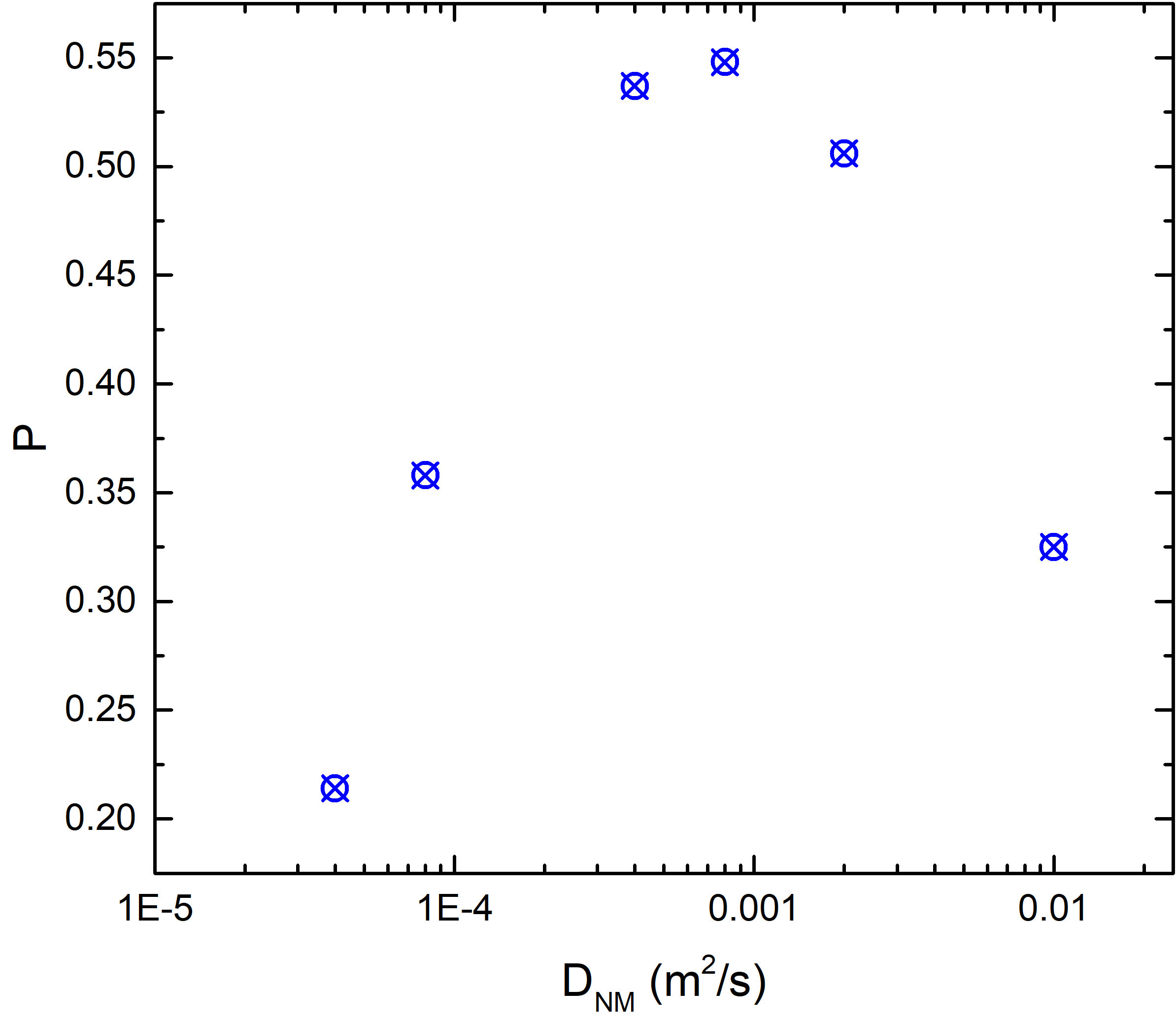
When the value of \(\lambda _{sf}\) in the contacts is reduced to 10 nm, however, diffusive effects start playing a bigger role: the extracted value of \(P\) is reduced to \(\sim 0.5\), so that it does not only represent the conductivity polarization \(\beta _\sigma \), but also depends on other system parameters. This is confirmed by using the drift-diffusion formalism to study the dependence of the extracted \(P\) on the diffusion coefficient in the NM layers \(D_\text {e,NM}\), reported in Fig. 7.6(b). It must be noted, that the present results are obtained in a symmetric structure, where RL and FL have the same length. In the presence of asymmetric FM layers, the angular dependence of the torque shows additional features [23], and an updated expression, which takes the diffusive effects into account, must be employed in order reproduce the torque dependence [152].

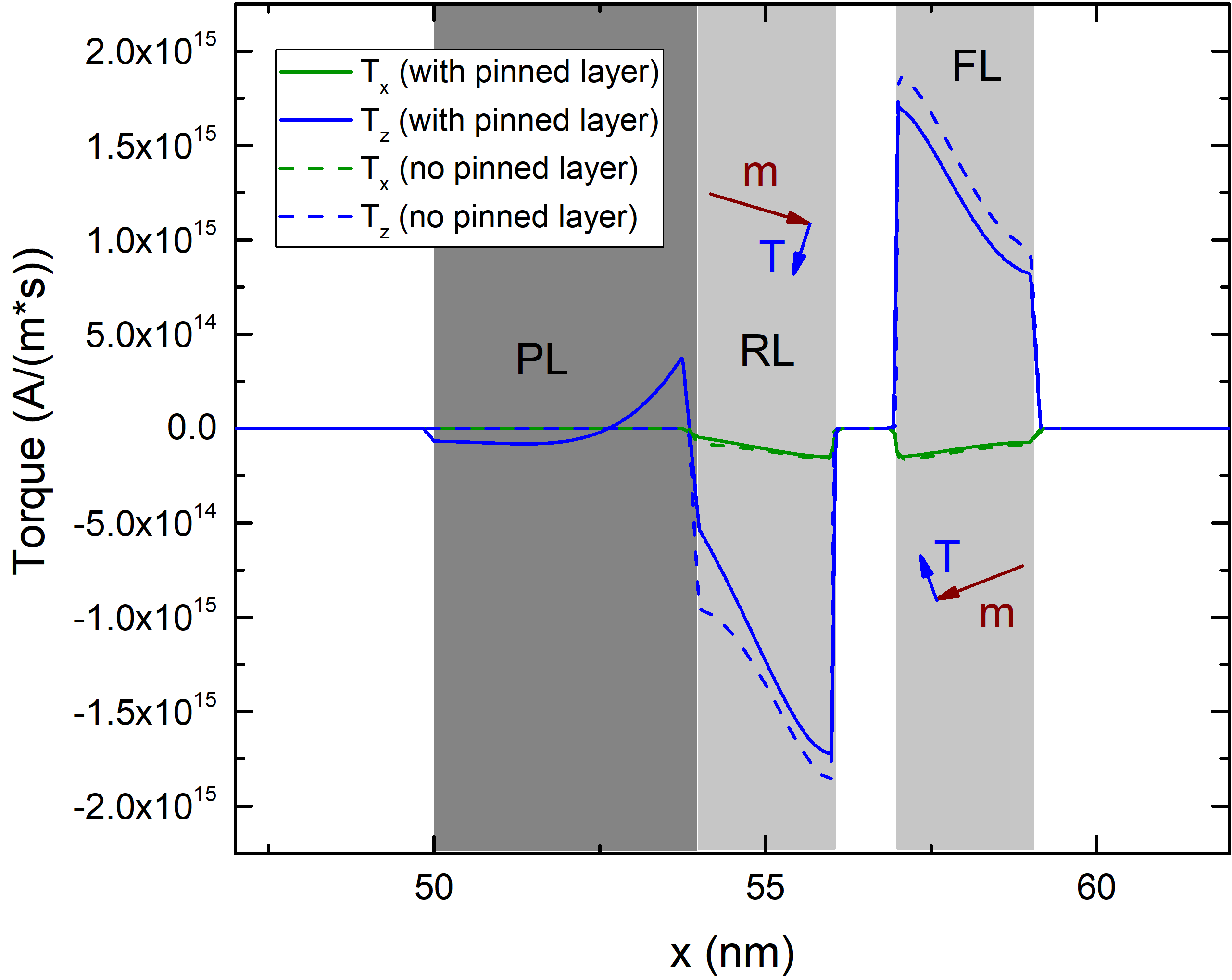
Even though the expressions for the average torque can be employed to simulate the magnetization dynamics of the FL, one of the main advantages of the drift-diffusion approach is the straightforward possibility to compute the torques acting in all the ferromagnetic layers in a given structure. This is particularly useful when the cell under study contains more layers than just the RL and FL. In [153], the writing failure of an MRAM cell at a high current density was linked to the destabilization of the RL. The torque acting from the FL back on the RL can become strong enough to cause the reversal of its magnetization, so that an equilibrium state of the cell is never reached. As seen in Chapter 2, the stability of the RL is usually increased by the presence of a pinning layer antiferromagnetically coupled to it. The effect on the torques acting in the structure in the presence of the additional PL is investigated. As the PL is usually a composite of multiple Co/Pd stacks with antiferromagnetic coupling [12], its polarization parameters are taken to be low, \(\beta _\sigma =\beta _\text {D}=0.1\). The length of the PL is 4 nm, and the spacer layer between RL and FL is 1 nm long. The magnetization is perpendicular to the plane of the structure, pointing along the positive x-direction in the RL and along the negative one in the PL.

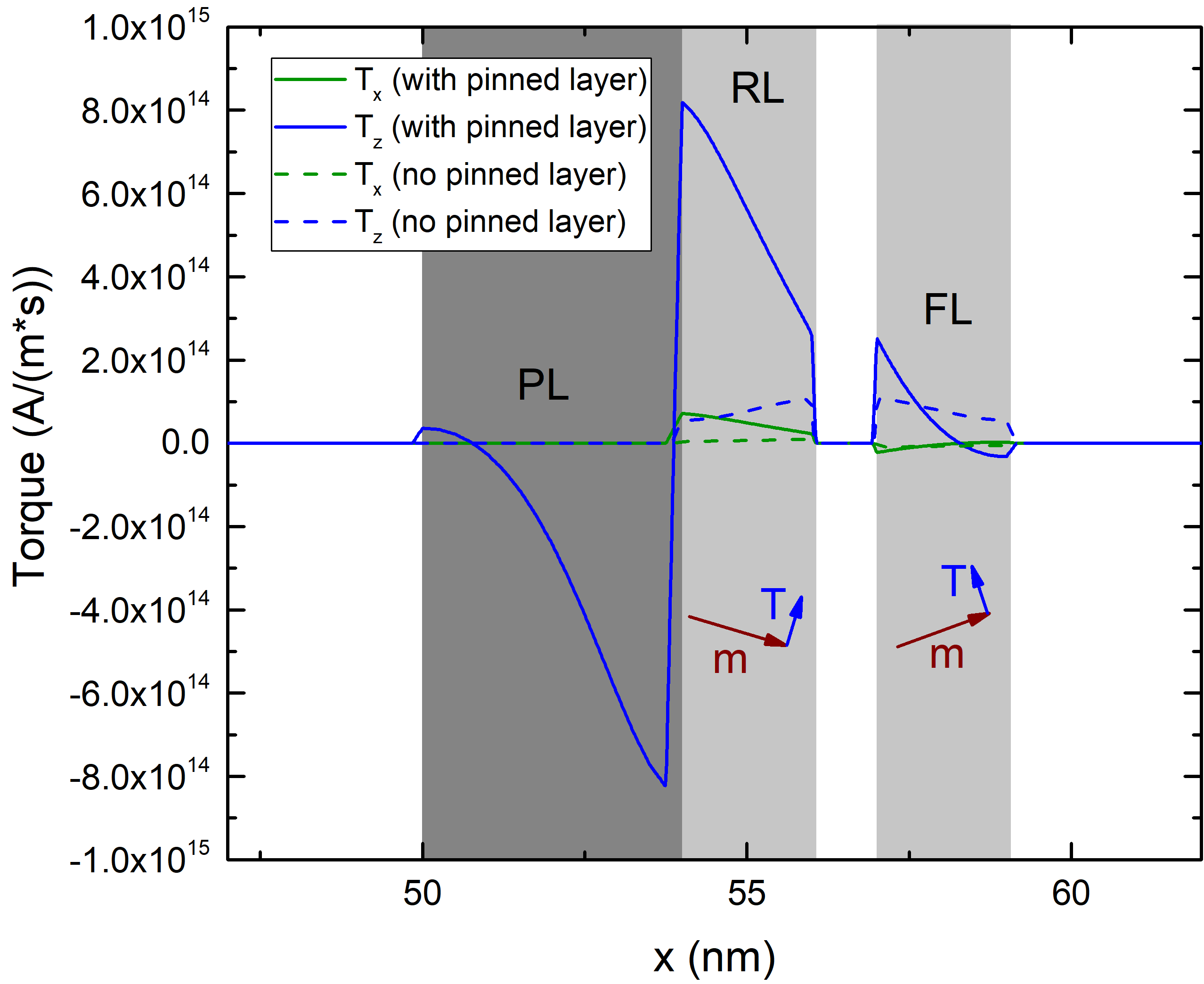
The components of the damping-like torque acting at the beginning of a P to AP simulation, with the magnetization of both RL and FL slightly tilted towards the z-axis, are reported in Fig. 7.7(a), compared to the ones acting in a structure without the additional PL. The presence of the pinning layer increases the torque pushing the magnetization to the x-axis, helping the stability of the RL. In Fig. 7.7(b) the torque acting at the end of the switching is reported. While the effect of the PL on the torque is less pronounced, its presence helps to partially reduce the torque destabilizing the RL at the end of the reversal process. These findings suggest that the presence of the PL, while increasing the stability of the RL thanks to the antiferromagnetic coupling, also affects the torque acting in the structure. The drift-diffusion implementation, having the possibility of computing the torque in the whole structure from a unified expression, allows to readily investigate the influence of additional FM and NM layers in modern MRAM cells.

7.4 Parameters Investigation for Reproducing the Torque in MTJs

The spin and charge drift-diffusion formalism was already successfully applied to the computation of the torques acting in a spin-valve structure with a metallic spacer layer [23]–[25]. However, most modern STT-MRAM cells are based on magnetic tunnel junctions. While the TMR effect on the charge current can be reproduced by employing (7.2), the spin accumulation solution needs also to be able to reproduce the expected magnitude, angular and voltage dependencies peculiar to MTJs [16], [99], [154]. In this section, the dependence of the spin accumulation on the material parameters entering the drift-diffusion equations is analyzed. It is shown how an effective choice of parameters is able to reproduce the torque magnitude and dependence on the polarization parameters predicted by Slonczewski [16]. The parameters employed for the simulations in this section are the ones reported in Table 7.1, unless differently stated.

In order to treat the middle layer as an ideal barrier with no spin reversal during the tunneling process, the spin-flip length \(\lambda _\text {sf}\) is taken to be infinite inside this layer. The equation for \(\vb {S}\) in the middle layer, where \(\vb {m}=\vb {0}\), reduces to

\begin{equation} \label {eq:SpinTunnel_SPIE} D_S\laplacian {\vb {S}} - D_\text {S}\frac {\vb {S}}{\lambda _\text {sf}^2}=0 \, , \end{equation}

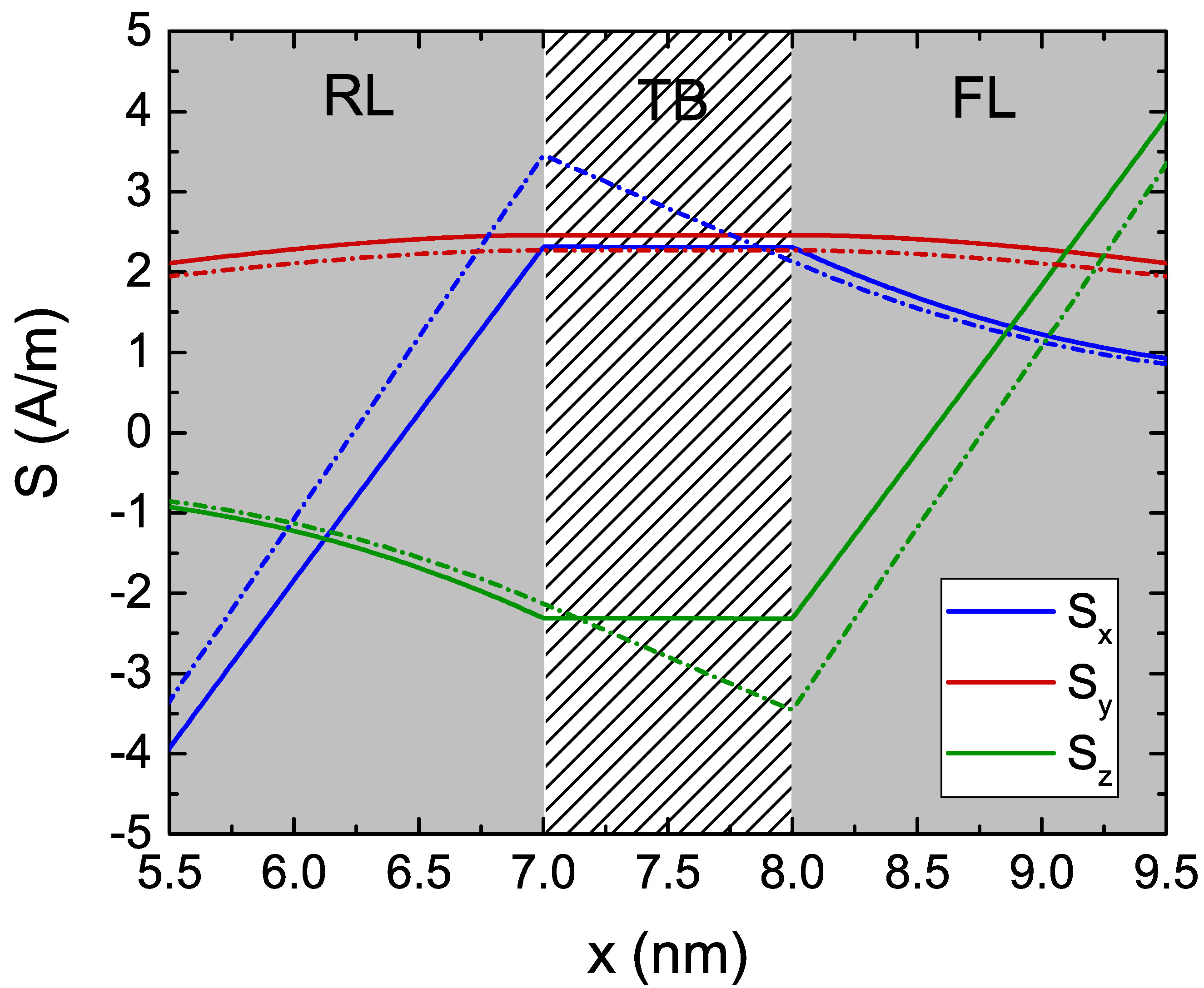
where \(D_\text {S}\) is the diffusion coefficient inside the barrier, and it is treated as a fitting parameter to be chosen properly in order to reproduce the torque behavior in an MTJ. Depending on its value, it can either increase or decrease the slope of the \(\vb {S}\) components in the middle layer. The effect of \(D_\text {S}\) on the spin accumulation behavior is reported in Fig. 7.8(a), for a structure with 5 nm long contacts, 2 nm long FM layers, and 1 nm long TB. A fixed current density flowing in the x-direction, perpendicular to the structure, is assumed, with value \(J_\text {C,x}=-10^{11}\) A/m\(^2\). The structure represents a pMTJ, with magnetization along x in the RL and along z in the FL. When the value of \(D_\text {S}\) is comparable to the one in the FM layers, the spin accumulation decays through the TB (dot-dashed lines), while the choice of a large spin diffusion coefficient reduces the slope in the middle layer to the point that the spin accumulation is practically preserved (solid lines). The solution in the whole structure for the high value of \(D_\text {S}\) is reported in Fig.7.8(b).

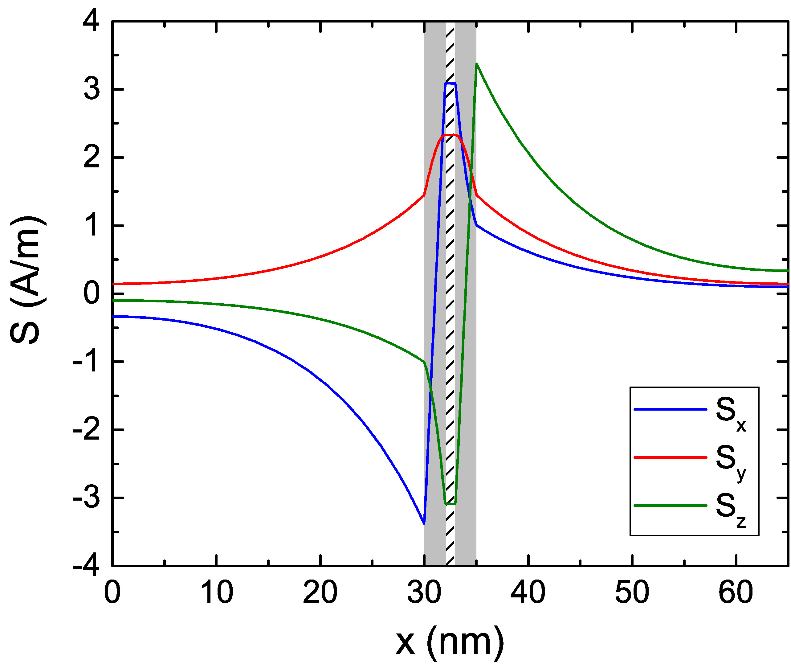
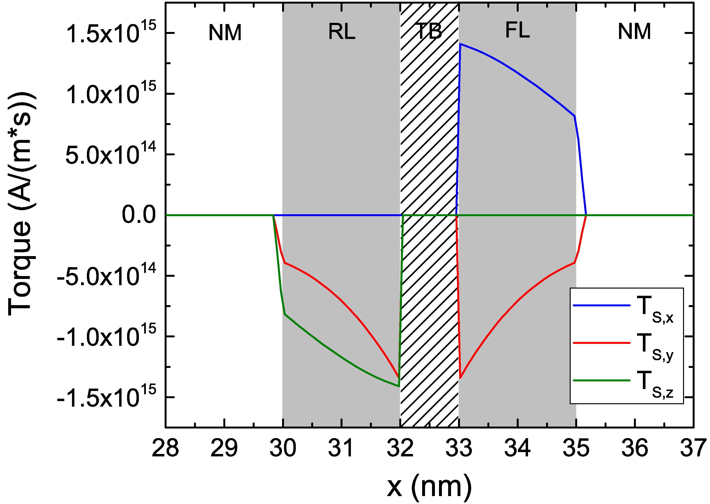
The non-magnetic leads are necessary, in a multilayer structure, to ensure decay of the spin accumulation inside the contacts. When they are sufficiently longer than the spin-flip length, all the spin accumulation components are able to fully relax to \(\vb {0}\), as reported in Fig. 7.9(a). The torque obtained from this solution of \(\vb {S}\) through (6.1) is reported in Fig. 7.9(b).

The dependence of the torque on the material parameters entering the spin accumulation equations (6.38) is then evaluated, in order to calibrate the model and to understand, if the choice of effective values for the parameters would be able to reproduce the STT torque predicted by Slonczewski [16]. The magnetization in the RL is set pointing in the x-direction, and the magnetization in the FL pointing in the z-direction. The employed structure has a squared cross-section of 40\(\times \)40 nm\(^2\), with ferromagnetic layers of 2 nm thickness and a middle layer of 1 nm thickness. The length of the non-magnetic leads is initially taken to be 5 nm. In Fig. 7.10, the obtained dependencies of both the adiabatic and non-adiabatic torque on several system parameters are reported. For these simulations, the same diffusion coefficient is used for all conducting layers, so that \(D_\text {e,NM}=D_\text {e,FM}\). The remaining non-varying parameters are taken from Table 7.1, unless differently stated.

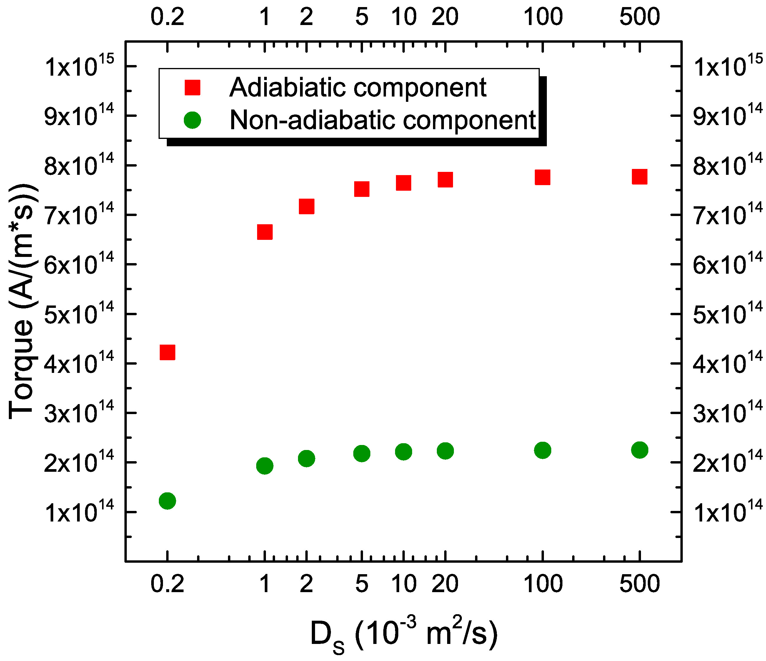
The dependence on the middle layer diffusion coefficient \(D_\text {S}\) is first analyzed. The results, reported in Fig. 7.10(a), show that the torques increase with the diffusion coefficient. The increase saturates at a value \(D_S=2.5\times 10^{-1}\) m\(^2\)/s, which is the one employed to compute the dependence on the other system parameters. This value of \(D_S\) is also the one preserving the spin accumulation across the middle layer in Fig. 7.8(a). Low values of \(D_\text {S}\), instead, increase the slope of the spin accumulation in the middle layer, and decrease the amount of spin-current transiting from one FM layer to the other, drastically reducing the torque.

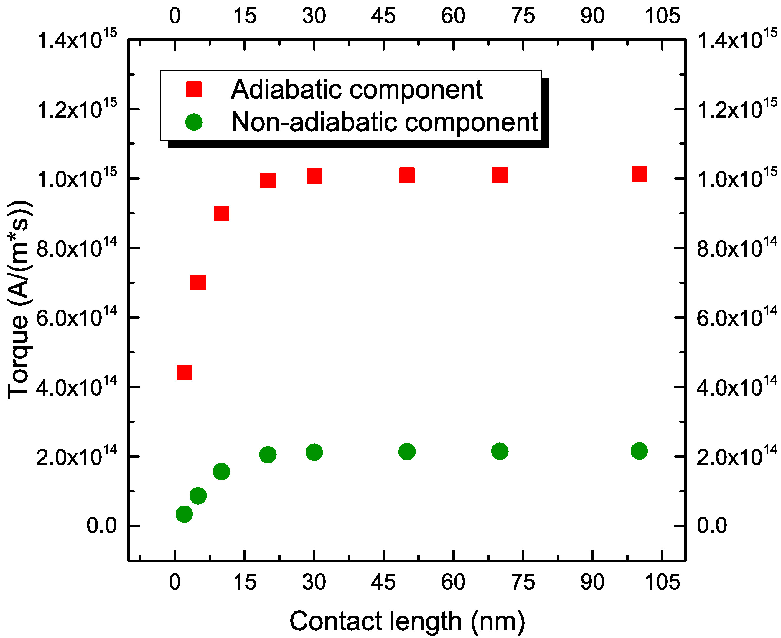
The dependence of the torques on the length of the NM contacts is subsequently analyzed. As already pointed out, due to the homogeneous Neumann boundary conditions applied to solve (6.38) with the FE approach, the solution can present a non-physical behavior, if the contacts included in the model are not long enough to allow the spin accumulation to completely decay [24], [25]. Fig. 7.10(b) reports the dependence of the torques on the length of the NM contacts. For the employed value of \(\lambda _\text {sf}\), a contact thickness of at least 30 nm is required to let \(\vb {S}\) relax to \(\vb {0}\) and obtain a torque value independent of this parameter. A structure with 50 nm contacts is employed for the remaining analysis.

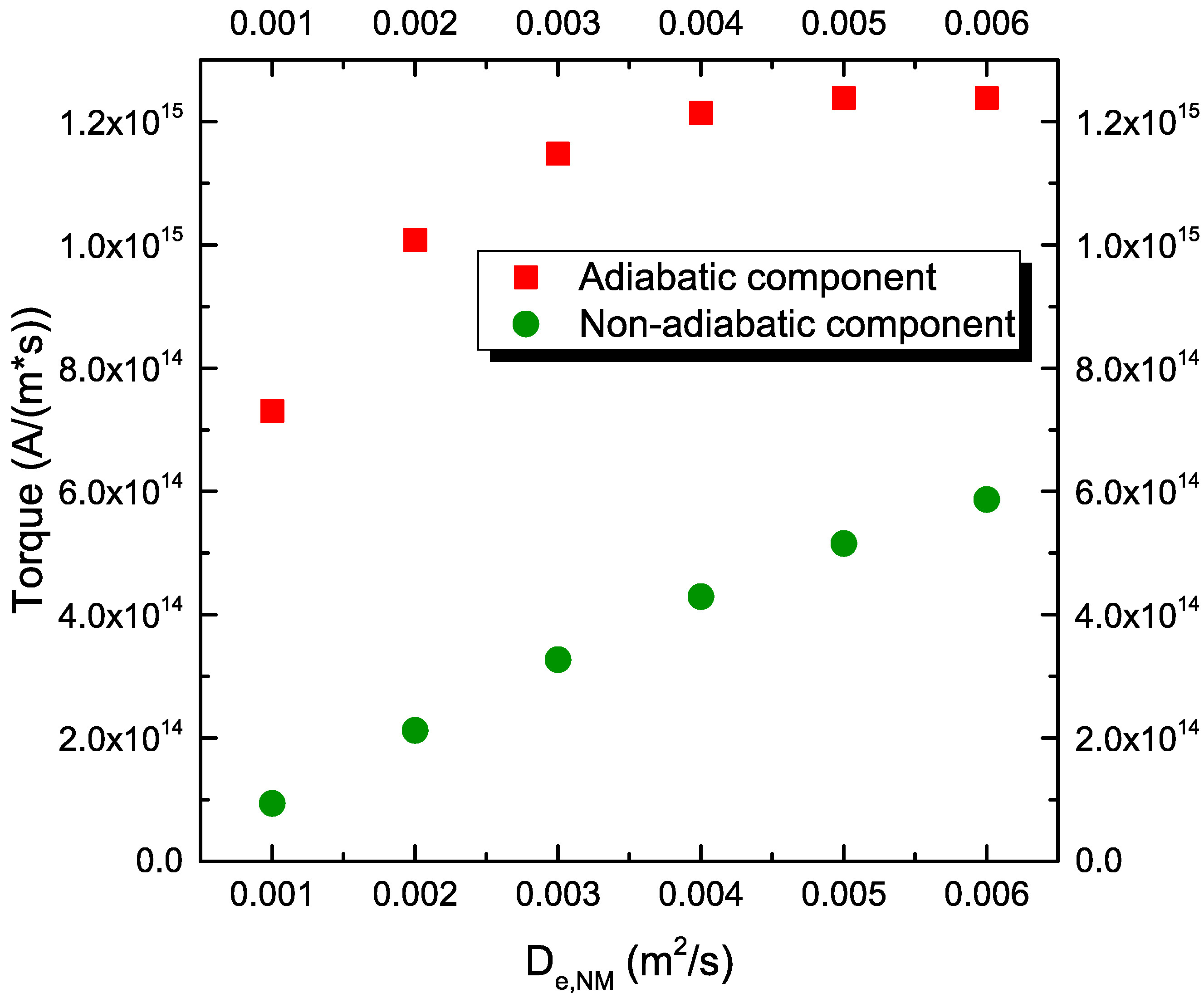
Fig. 7.10(c) reports the dependence on the magnitude of the diffusion coefficient in the NM contacts, showing that, even if the exchange between the magnetization and the spin accumulation happens in the ferromagnetic layers, this parameter still has an effect on the torque magnitude, due to the continuous nature of the spin accumulation in the presented formalism. When \(D_\text {e,NM}>D_\text {e,FM}\), the balance of diffusion and magnetization change at the FM/NM interface allows for a better polarization of the current, increasing the total amount of torque transferred to the magnetization.

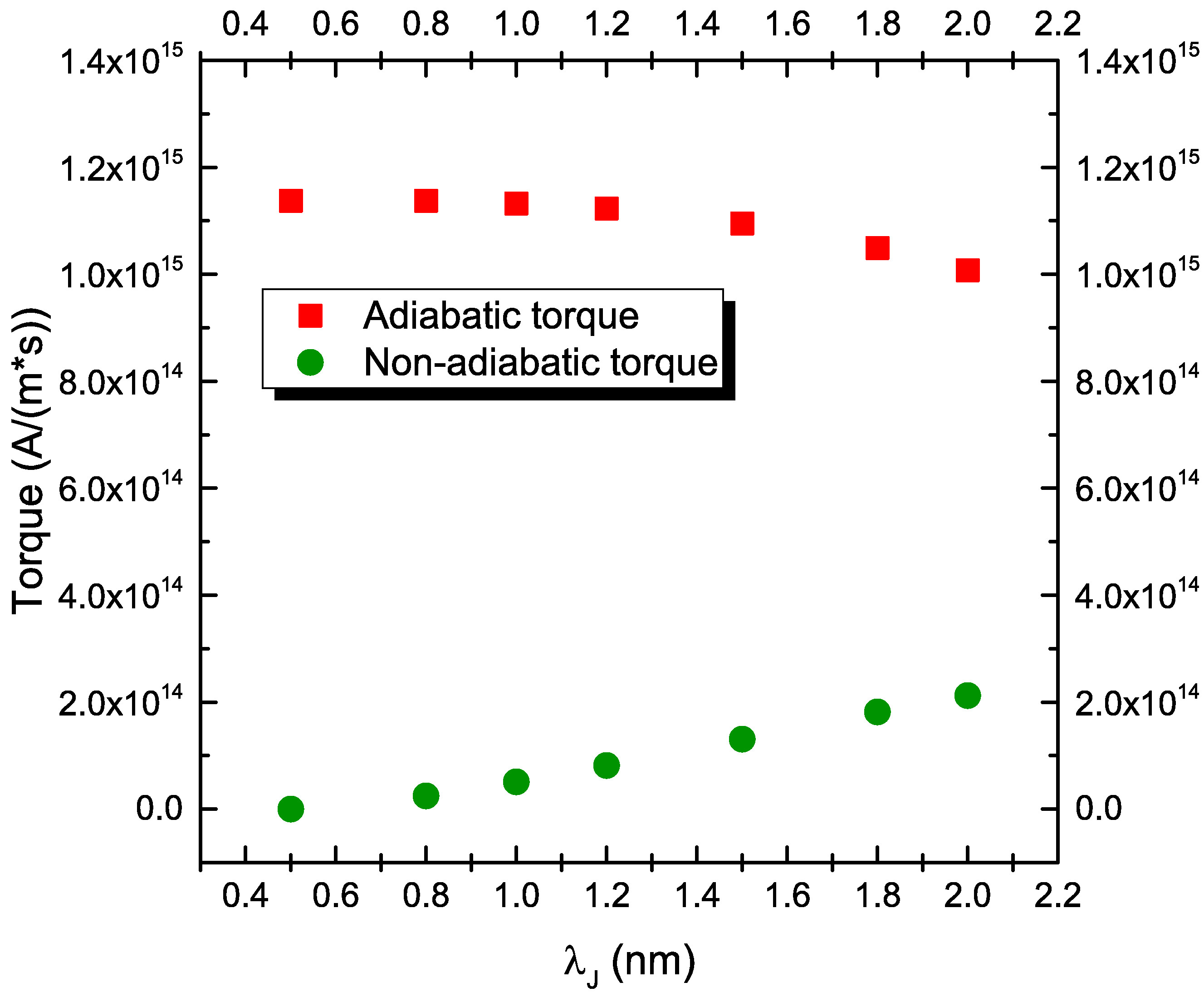
Fig. 7.10(d) then reports the dependence on the value of the exchange length. Lower values of \(\lambda _\text {J}\) imply a stronger exchange coupling, and produce an increased adiabatic torque. They also change the relative importance of the non-adiabatic component coming from the drift-diffusion formalism. A shorter \(\lambda _\text {J}\) implies a faster absorption of the transverse components of \(\vb {S}\), so that values below 1 nm bring these components to almost 0 in the space of the FL.

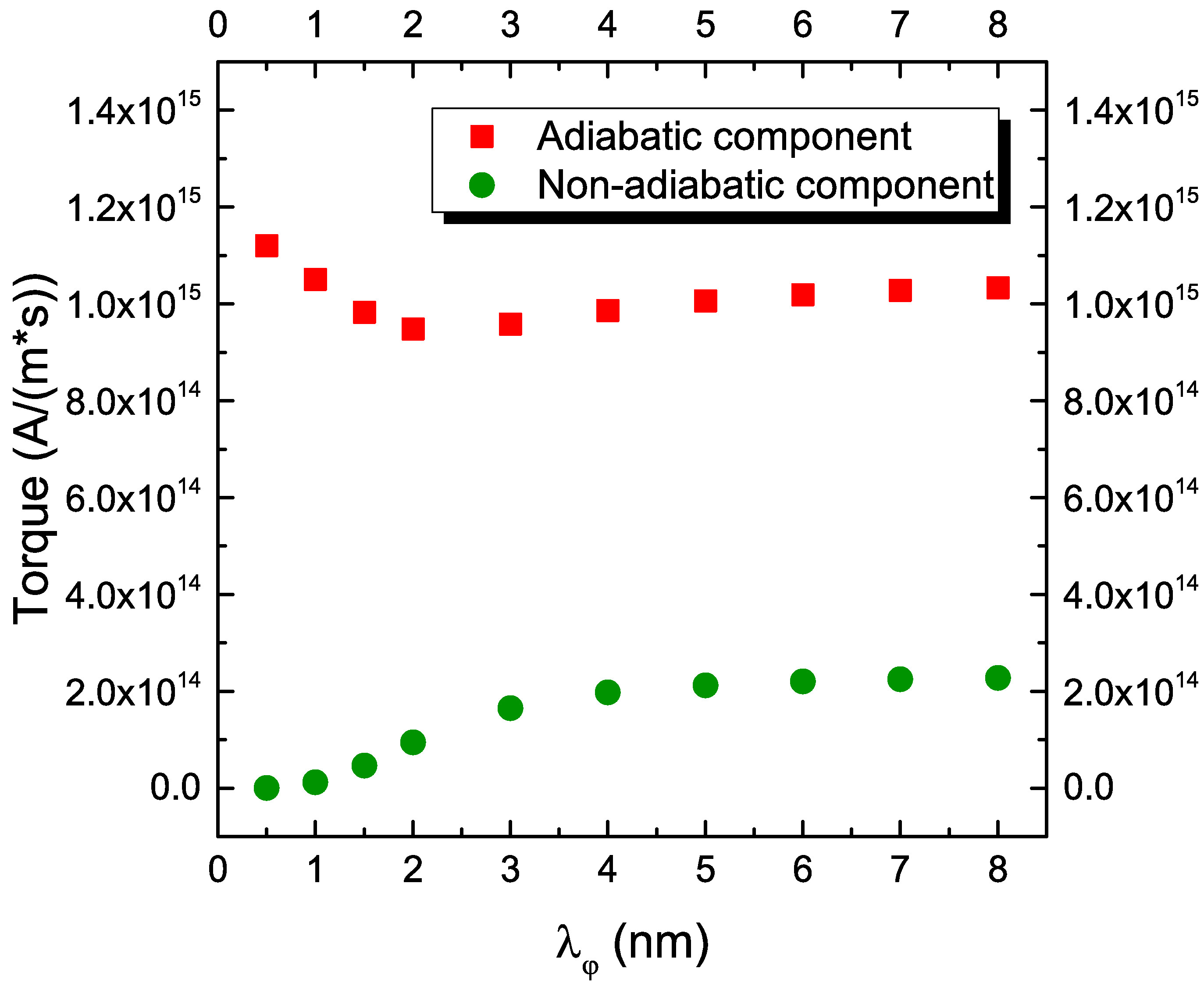
The influence of the spin dephasing length \(\lambda _{\varphi }\) on the computation of the torque is also investigated. Results are reported in Fig. 7.10(e). For values of \(\lambda _{\varphi }\) less than 3 nm, its contribution to the torque is substantial. This suggests that, when the value of \(\lambda _{\varphi }\) is close to \(\lambda _\text {J}\), the effects of the former have to be taken into consideration for accurately describing the magnetization dynamics.

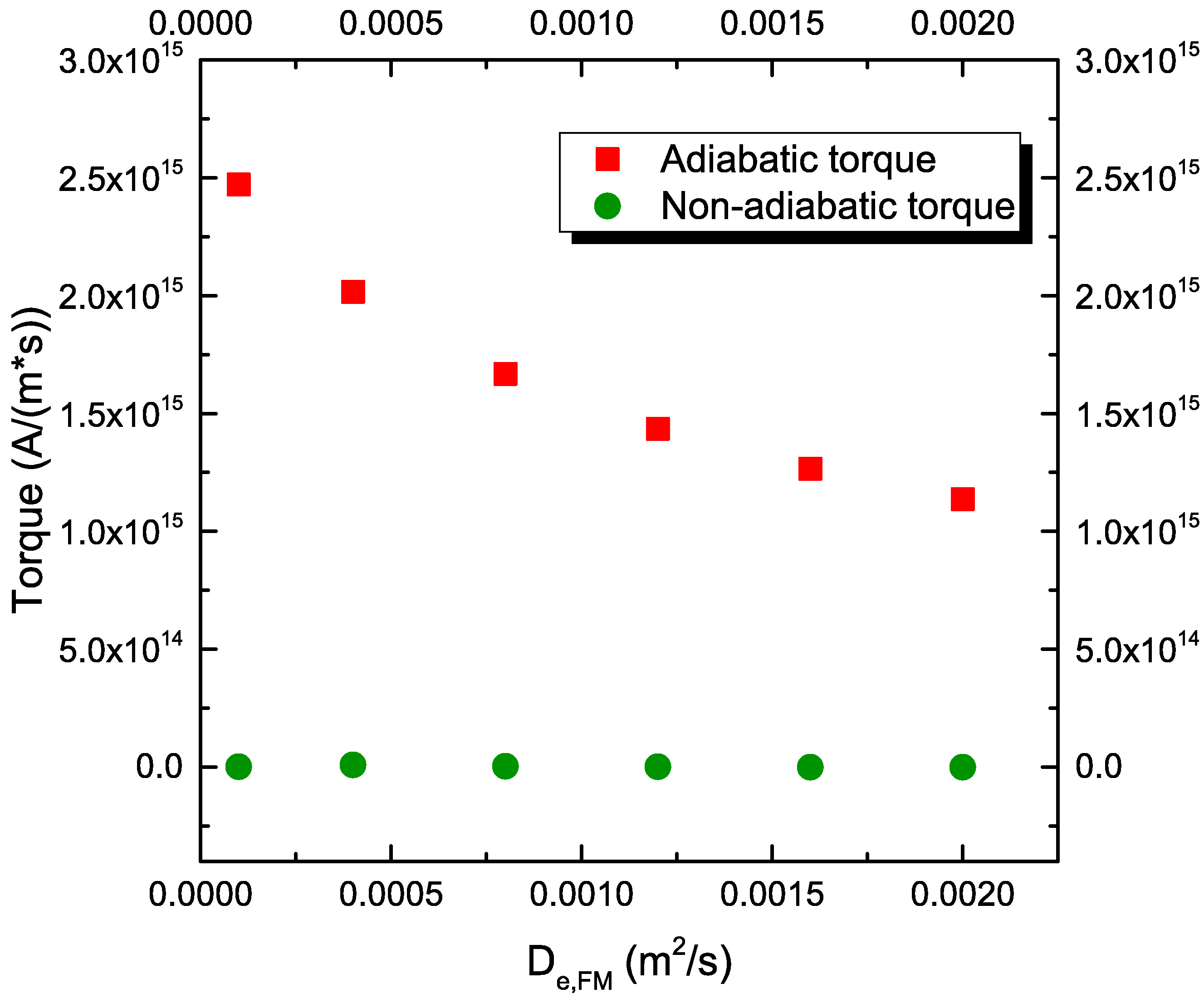
Finally, Fig. 7.10(f) reports the dependence of the torque on the diffusion coefficient of the FM layers. For this plot, an exchange length \(\lambda _\text {J} = 0.5\) nm is employed, which lets the transverse components of \(\vb {S}\) be entirely absorbed. The results show that a lower value of \(D_\text {e,FM}\) increases the magnitude of the adiabatic torque, as the first term in equation (6.38), describing the magnetization dependent polarization of the electric current, becomes dominant over diffusive effects, allowing for the spin current to reach the value of \(-(\mu _\text {B}/e)\beta _\sigma \vb {J}_\text {C}\).

The torque dependencies reported until now considered only one parameter at a time. While this gives an idea of how the torques react to changes in the considered coefficients, possible interdependencies between them could be overlooked. The behavior of the damping-like torque component under changes in several combinations of the involved length and diffusion constants is thus also investigated.

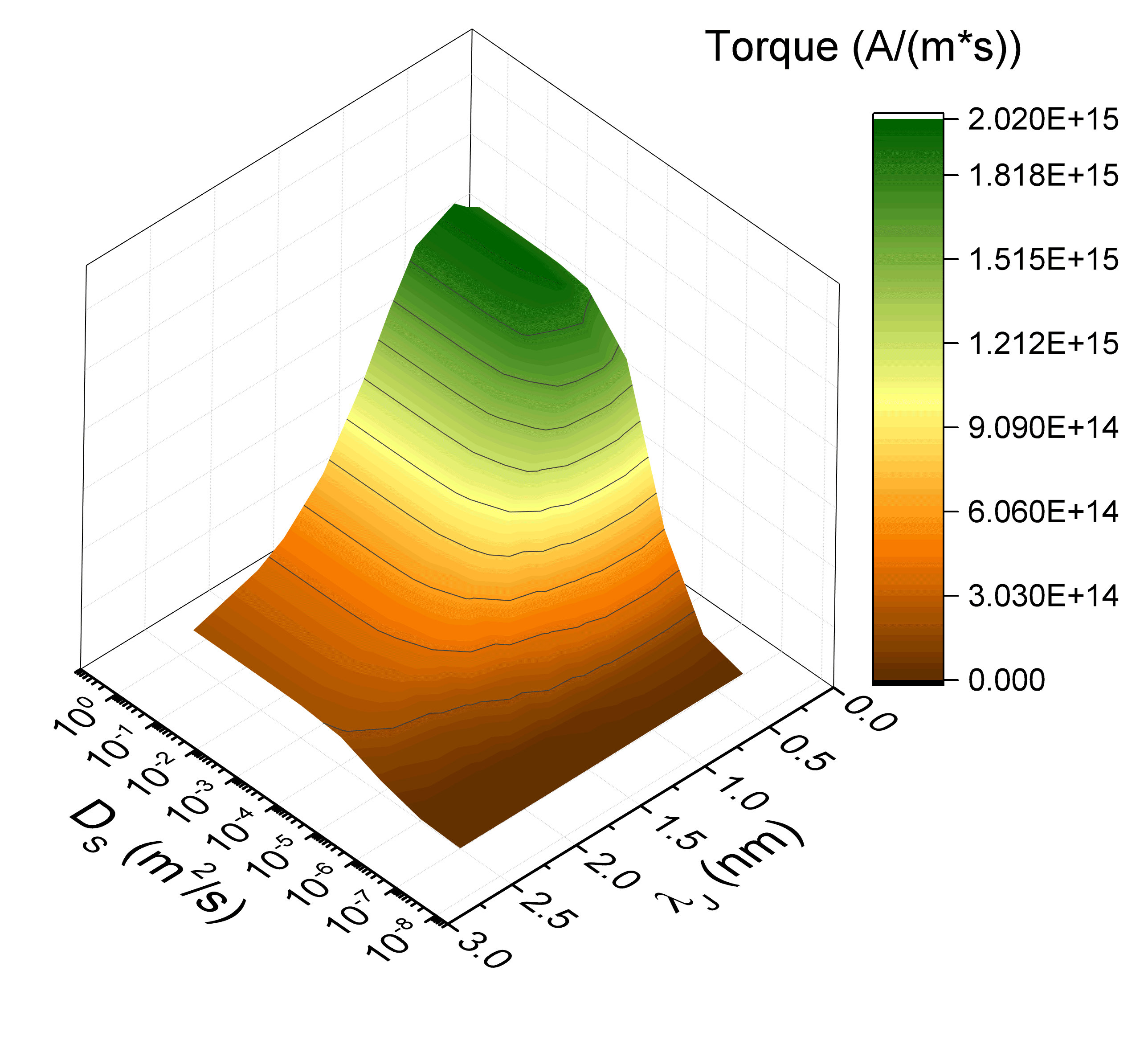
In Fig. 7.11(a) the dependence of the average value of the damping-like torque on the exchange length \(\lambda _\text {J}\) and on \(D_\text {S}\) is reported. As observed before, low values of \(D_\text {S}\) greatly reduce the torque, while high values enhance the torque, for every value of \(\lambda _\text {J}\). Regardless of the value of \(D_\text {S}\), the torque is enhanced by lower values of \(\lambda _\text {J}\), as they allow the transverse components of the spin accumulation to be completely absorbed in the space of the FL.

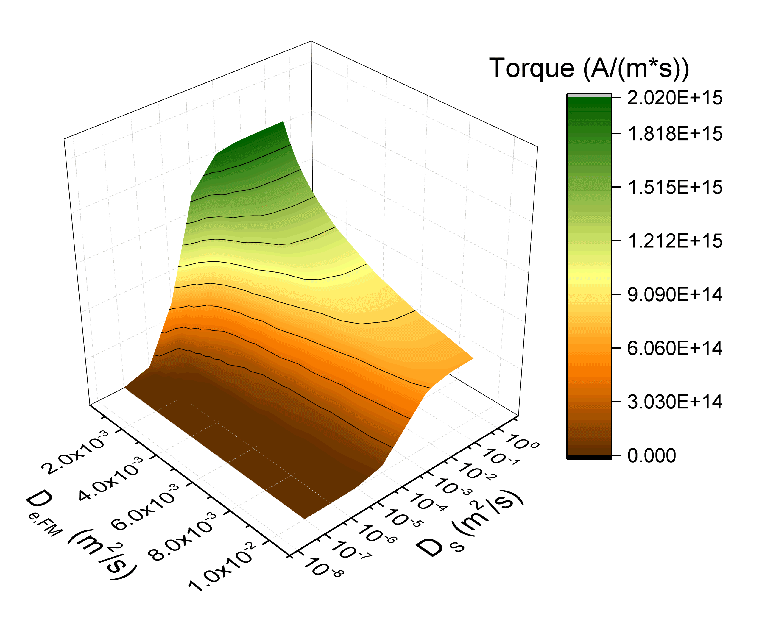
Fig. 7.11(b) reports the dependence on \(D_\text {S}\) and on the diffusion coefficient of the FM layers \(D_\text {e,FM}\). For high values of \(D_\text {S}\), the torque increases as \(D_\text {e,FM}\) decreases, as observed in the previous analysis, while the lower values of \(D_\text {S}\) reduce the torque to the point that its dependence on \(D_\text {e,FM}\) also becomes less evident.

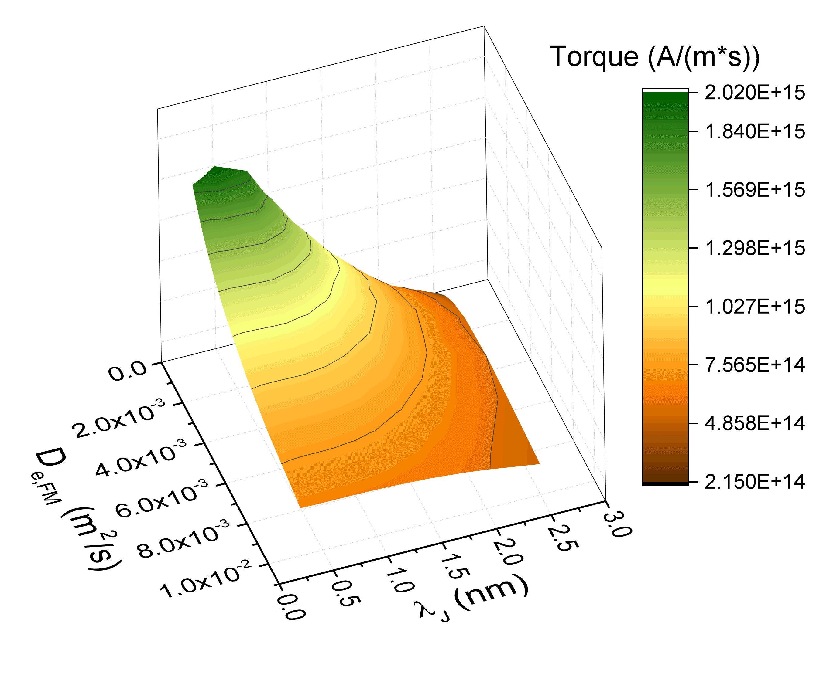
Fig. 7.11(c) reports the dependence on the diffusion coefficient of the FM layers, \(D_\text {e,FM}\), and on \(\lambda _\text {J}\). As the torque equation (6.1) depends on the ratio of these two parameters, the interplay between them is such that a lower \(D_\text {e,FM}\) both enhances the torque, as observed before, and makes it more dependent on the exact value of the exchange length.

The dependence of both the FL and RL adiabatic torque component on the RL conductivity polarization is investigated in Fig. 7.12(a). For this plot, values of \(D_\text {e,FM}=10^{-4}\) m\(^2\)/s and \(\lambda _\text {J}=0.5\) nm are employed. The torque on the FL shows a linear dependence on this parameter, while the torque on the RL is almost independent of it.

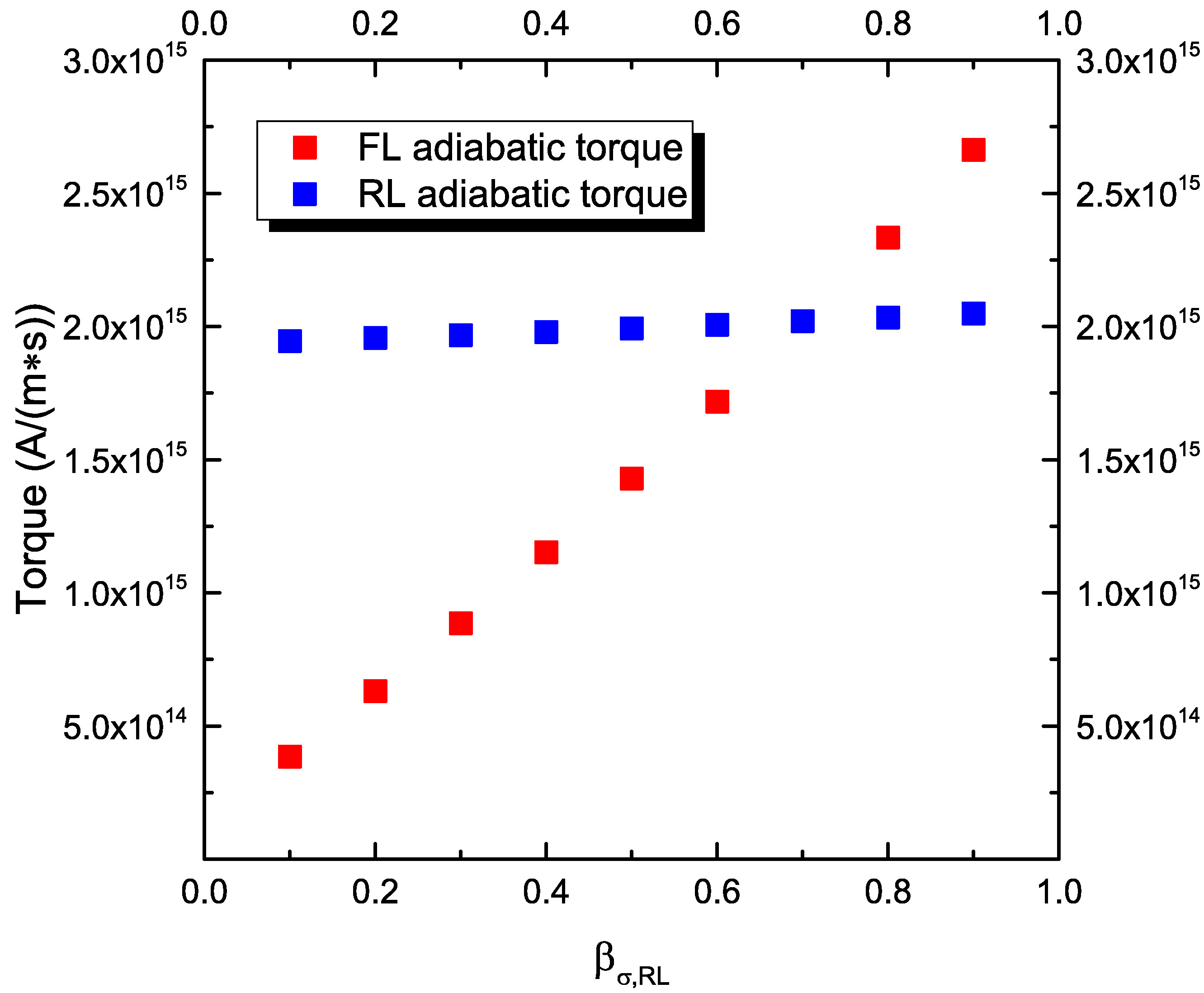
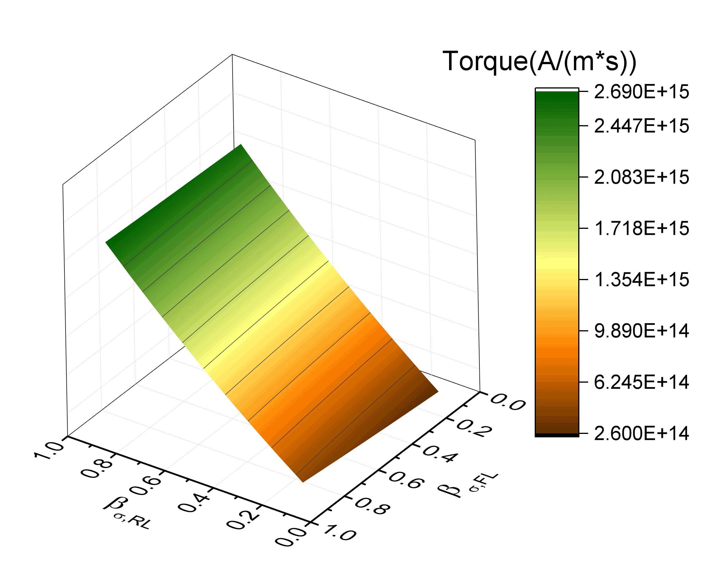
Fig. 7.12(b) then shows the dependence of the FL adiabatic torque on the conductivity polarization of both the RL and FL. For any value of \(\beta _{\sigma \text {,FL}}\), the value of the torque in the FL still shows the same linear dependence on the polarization of the RL, and it is almost constant with respect to the one of the FL. This behavior is compatible with the dependence on \(P_\text {RL}\) and \(P_\text {FL}\) expected from the adiabatic component of the Slonczewski torque term in (3.47), which, for the FL of the structure under study, takes the form

\begin{equation} \vb {T}_\text {S} = \frac {g \mu _B J_\text {C,x}}{e M_S d_\text {FL}} \, \frac {P_\text {RL}}{2 \pqty {1 + P_\text {RL}\,P_\text {FL} \cos \theta }} \, \vb {m}_\text {FL}\cross \pqty {\vb {m}_\text {FL}\cross \vb {m}_\text {RL}} \, , \label {eq:torque_slonc} \end{equation}

where \(\theta \) is the angle between \(\vb {m}_\text {RL}\) and \(\vb {m}_\text {FL}\), so that \(\cos \theta = \vb {m}_\text {RL}\vdot \vb {m}_\text {FL}\). With \(\theta =90^{\circ }\) and \(P_{RL}=P_{FL}=0.7\) (giving a TMR of \(\sim 200\)% from (3.51)), this produces a damping-like (DL) torque in the FL of \(T_\text {S,DL}=2.03 \times 10^{15}\) A/(m s). 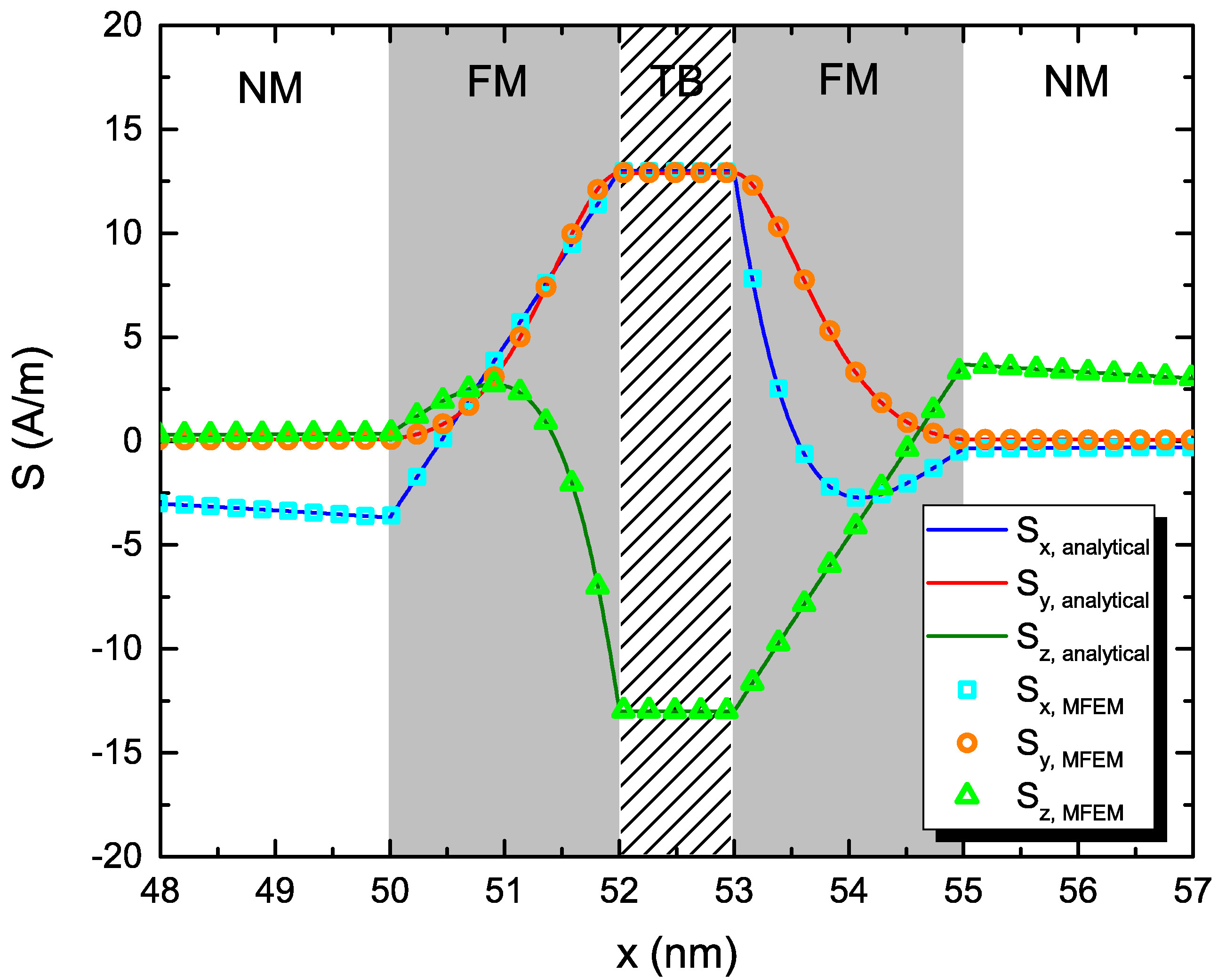The previous analysis can be employed to calibrate the torque produced by the FE drift-diffusion solver and extract a set of effective parameters capable of reproducing the one predicted by the Slonczewski term. In Fig. 7.13(a) the spin accumulation solution for the modified set of parameters reported in Table 7.2 is shown. 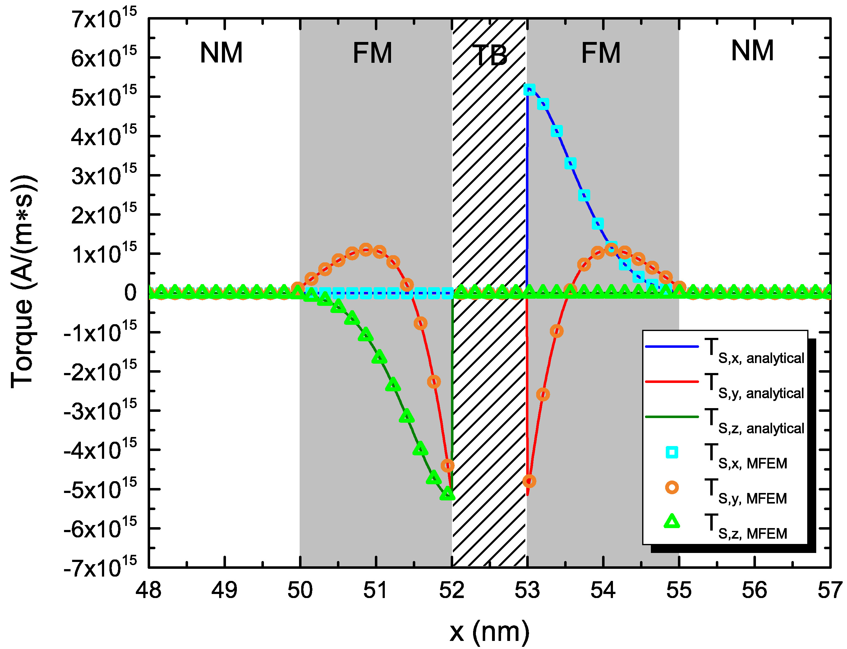The lower exchange length allows the transverse components of \(\vb {S}\) to be completely absorbed inside the FL, as typically expected for strong ferromagnets [16], [155], while the lower value of the diffusion coefficient in the ferromagnetic layers allows the polarization term in (6.38) to dominate the spin current value. The torque acting on both ferromagnetic layers is reported in Fig. 7.13(b). The solution computed through the solver is compared to one based on analytical expressions for the spin accumulation in the different layers, obtained by including the \(\lambda _{\varphi }\) term to the results presented in [156] and adapting them to the structure under study. The resulting system of equations is reported in Section A.1 of the Appendix. The two results are in perfect agreement, confirming the accuracy of the FE solver. The average damping-like torque acting on the FL obtained from (7.4) is \(T_\text {S,DL} = 2.02 \times 10^{15}\) A/(m s), which is compatible with the value computed using (7.6). The drift-diffusion approach, thanks to the presented effective choice of material parameters, is thus able to reproduce the torque magnitude expected in MTJs.

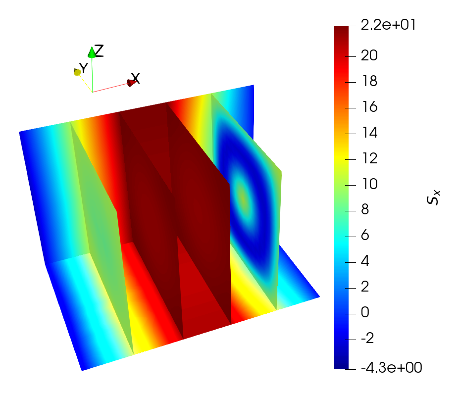
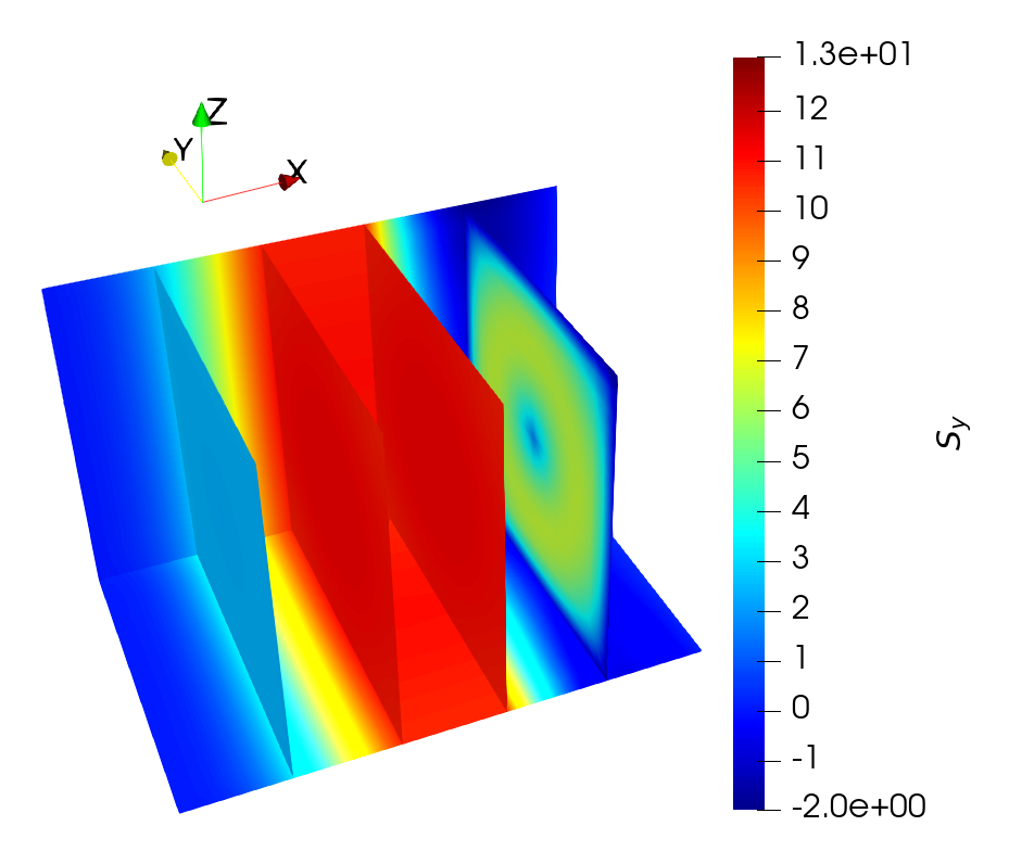
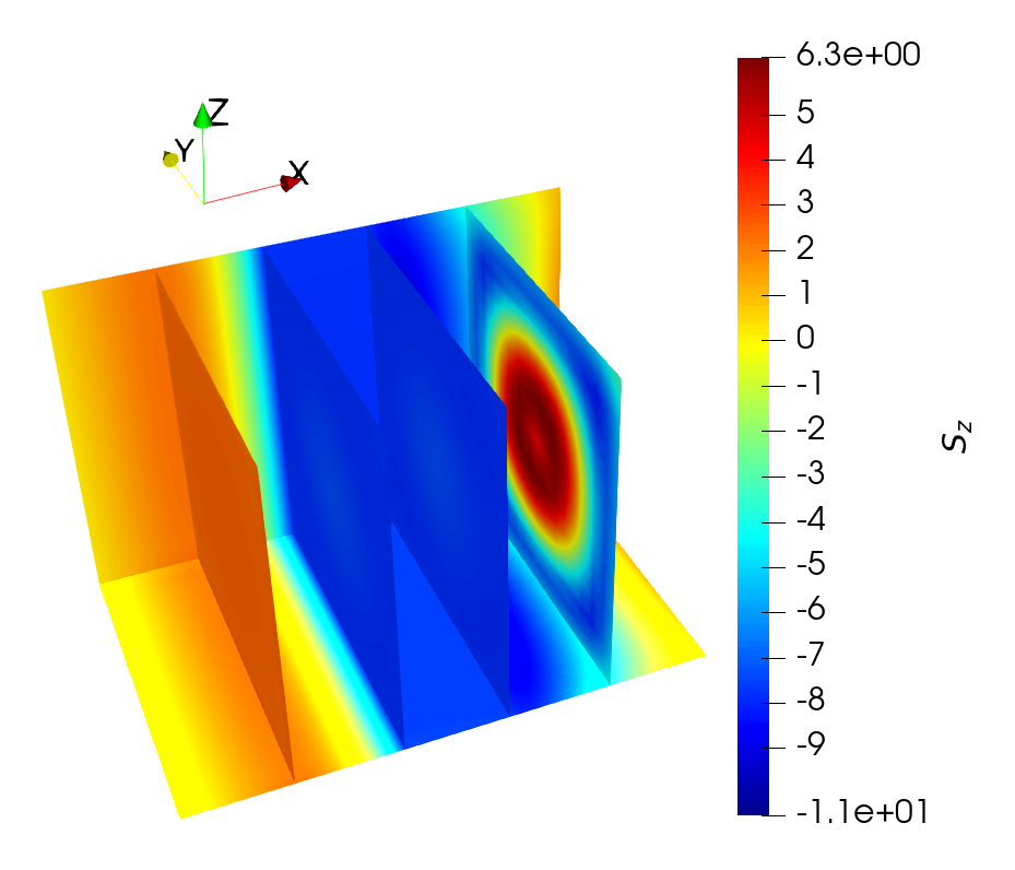
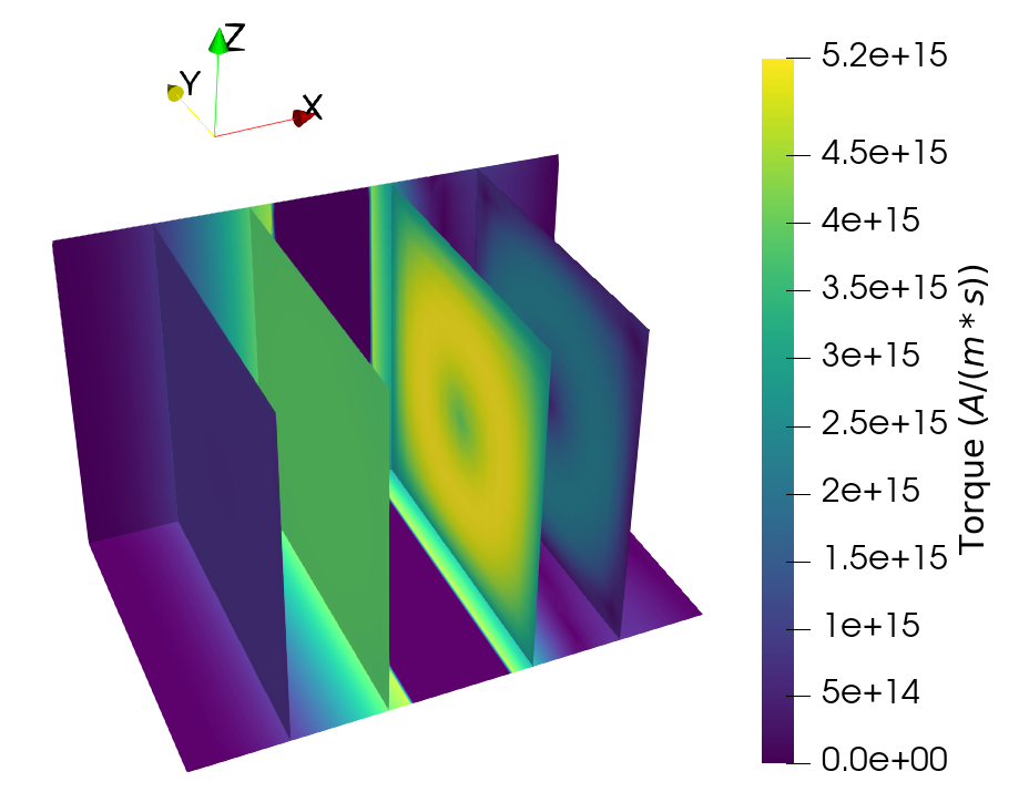
The advantage of the FE implementation over the presented analytical solution is the possibility to compute \(\vb {S}\) in more articulated structures and with non-uniform magnetization configurations, typical during the switching process. The three components of a three-dimensional solution for the spin accumulation, computed using the parameters in Table 7.2 and the same magnetization configuration, MTJ conductance and TMR employed for the results in Fig. 7.1, is reported in Fig. 7.14. The structure is sandwiched by 50 nm NM contacts. The applied bias voltage is \(-3.36\) V, producing a current density \(J_\text {C,x}=-10^{11}\) A/m\(^2\) at \(\theta =90\)°. The spin accumulation is redistributed, in both layers, in response to both the nonuniform magnetization configuration and the current density distribution. This solution, computed using (6.60), (6.59) and (7.2), can be plugged into (6.58a) for computing the torque and evaluating the magnetization dynamics.

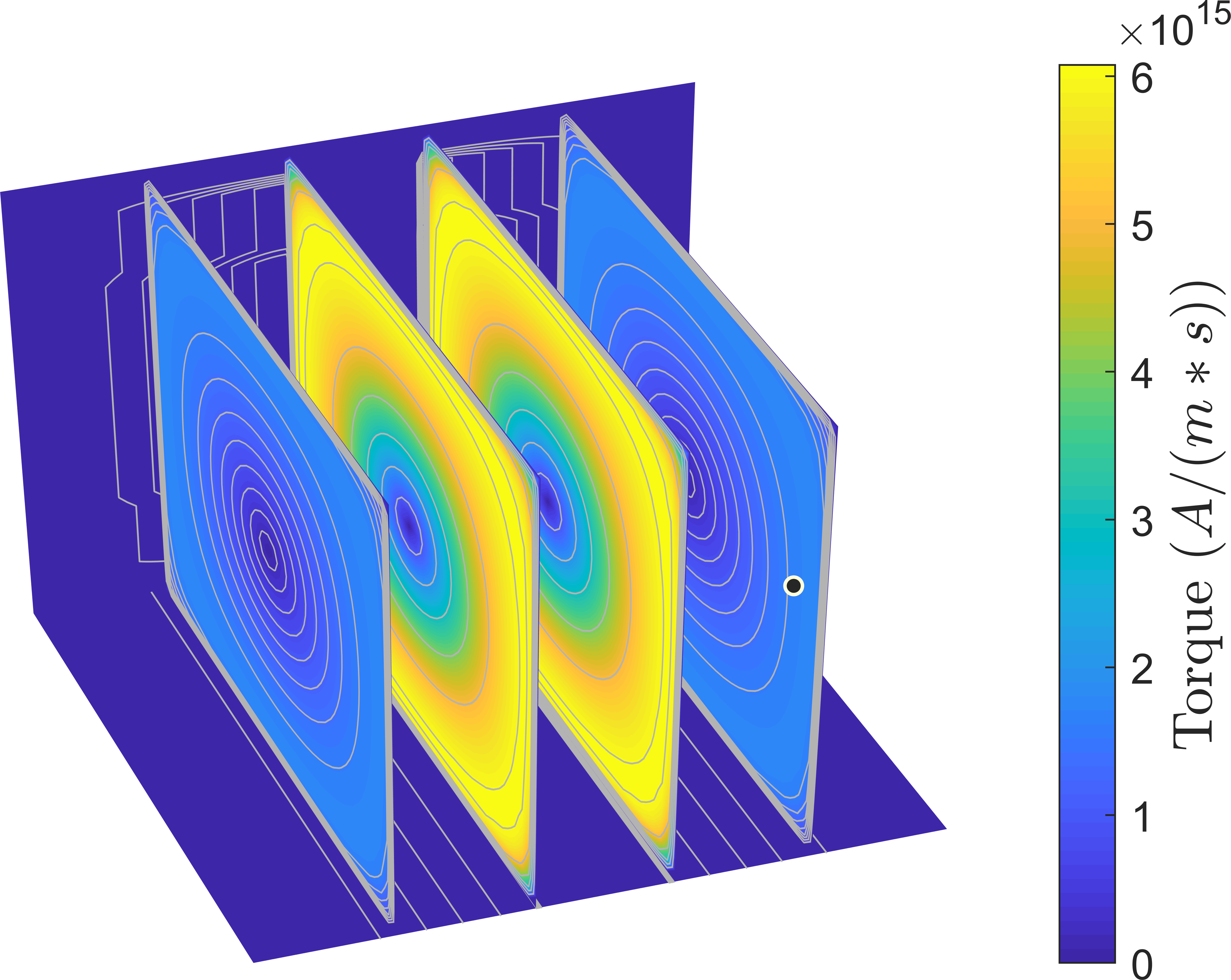
Moreover, the difference between the torque computed from a combination of analytical solutions at various angles and the fully three-dimensional one is investigated. The solutions for the torque obtained from the analytical expression at several values of \(\theta \) were combined into a single image, matching the magnetization distribution showcased in Fig. 4.1. The damping-like component’s magnitude for the combined torque is reported in Fig. 7.15(a). The one for the torque obtained from the spin accumulation of Fig. 7.14 is shown in Fig. 7.15(b). It can be seen that the analytical approach fails to account for the redistribution of \(\vb {S}\) due to diffusive effects and local gradients in the magnetization, so that the full solution computed by the FE solver can better capture the torque acting on the magnetization.

7.4.1 Limitations of the Effective Parameters’ Approach

The results presented in this chapter show that it is possible to employ effective material parameters to obtain a spin accumulation with the right sign and magnitude to reproduce typical values of the STT torque expected in an MTJ. The FE approach to the drift-diffusion formalism gives the possibility of computing the torques in all the ferromagnetic layers of the structure for a variety of three-dimensional meshes. It must be noted, however, that the presented approach is not sufficient to reproduce all the properties of the MTJ torque. The first right hand side term of equation (6.60) poses a strictly linear dependence of the torque on the applied bias voltage, coming from the linear dependence of \(\vb {J}_\text {C}\) on \(V\) from equation (6.59). Theoretical calculations [99], [154], [157], [158] and experimental findings [159]–[162] have shown that, at high bias voltage, the adiabatic component can present a nonlinear behavior, while the non-adiabatic component is symmetric with respect to the applied bias.

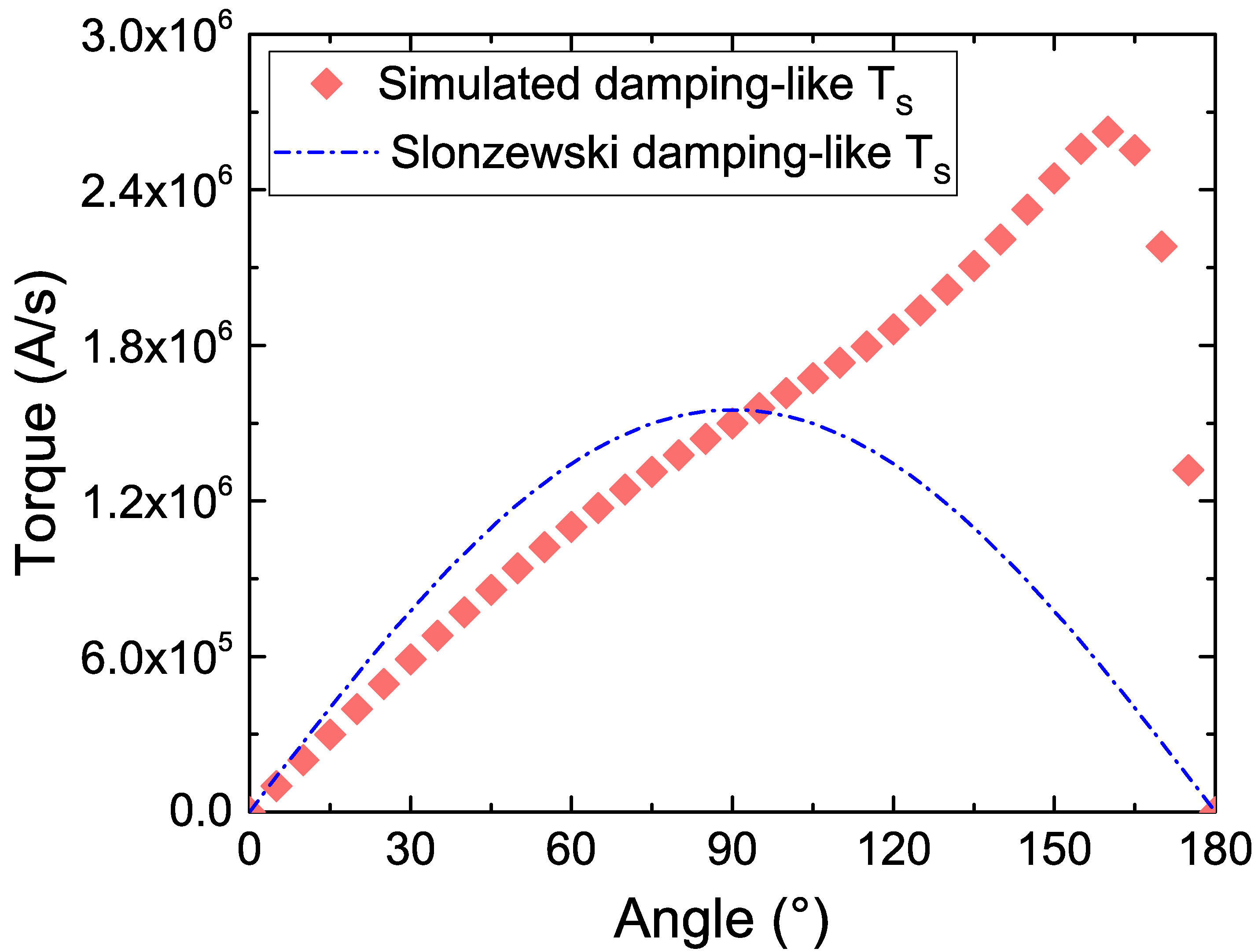
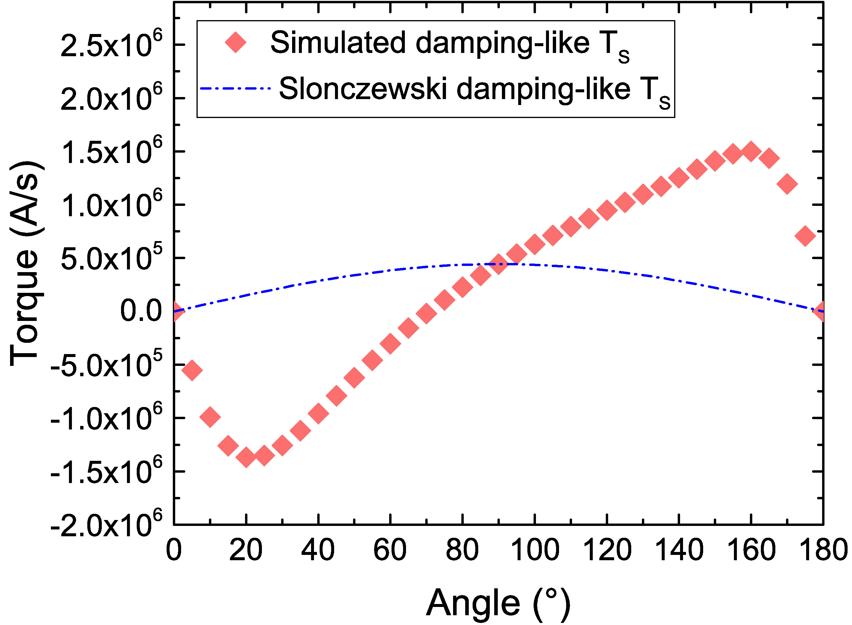
Moreover, the angular dependence of the torque obtained by the presented formalism diverges from the sinusoidal one predicted in MTJs under a constant bias voltage [16], [99]. In Fig. 7.16(a), the angular dependence of the damping-like torque acting on a semi-infinite FL is compared with the Slonczewski expression (7.6). \(J_\text {C,x}\) is extracted from the FE charge current solution for every value of the angle \(\theta \). For these results, semi-infinite FM layers are considered, to exclude any influence of the FL length and of the NM contacts, and a constant bias voltage of \(V=-1.3\) V is applied. Because of the constant bias, the dependence of (7.6) on the angle is given only by \(\sin \theta \), in contrast to the dependence at a constant current and current density, where the \(\cos \theta \) term in the denominator plays a role. The reported values are obtained from the torque integral (7.4) without the division by the FL thickness. While the torques obtained at \(\theta =90\)° are compatible, thanks to the previous calibration, there is a clear deviation of the drift-diffusion results from the expected ones at other values of \(\theta \). A modification in the polarization parameters can also have a huge impact on the angular dependence. In Fig. 7.16(b), results for \(\beta _{\sigma ,\text {RL}}=0.2\) are reported, compared to the Slonczewski results for \(P_\text {RL}=0.2\). In this case, the discrepancy between the drift-diffusion results and the Slonczewski ones is even greater, with the torque computed by the former changing its sign for \(\theta < 75\)°. Negative values of the torque indicate that it is favoring the anti-parallel orientation of the layers, rather than the parallel one. This wavy torque behavior has been reported and studied in metallic valves [125], but is not typical of MTJs. In order to employ the approach presented in this chapter to obtain a sinusoidal angular dependence, characteristic to MTJs, several independent sets of angular-dependent parameters are needed for different relative orientations of the magnetization vectors. As this procedure is clearly unacceptable, a more appropriate treatment of the tunneling spin-current is thus required to be able to comprehensively reproduce the properties of the torque acting in MTJs. A suitable approach will be developed in the next Chapter.