Computation of Torques
in Magnetic Tunnel Junctions
Chapter 8 Tunneling Spin Current in the Drift-Diffusion Formalism and Applications to Ultra-Scaled MRAM Switching Simulations
The drift-diffusion approach previously described only accounts for semi-classical transport properties, and needs to be adapted to the description of the tunneling process across an MTJ. While the TMR effect can be reproduced by
describing the TB conductivity through (7.2), using effective material parameters for the spin equation is not sufficient to reproduce all the expected
torque properties. This chapter shows how the FE solver must be enhanced with appropriate boundary conditions at the TB interfaces to account for the tunneling spin current. It is shown how both the angular and voltage
dependencies expected in MTJs are reproduced by the presented approach, which also predicts an interdependence between the torque acting in the presence of magnetization gradients and the tunneling spin current. The solver is
then applied to simulate the magnetization dynamics of ultra scaled multi-layered structures with composite ferromagnetic layers. The results hereby presented were published by the author in references [163],[164], and [13].
8.1 Spin Drift-Diffusion Extension to Include MTJ Properties
The drift-diffusion (DD) approach described in the previous chapter needs to be updated to incorporate the effect of the tunneling process on the spin accumulation. In order to do this, an appropriate expression for the tunneling
spin current needs to be included in the model. The Nonequilibrium Green Functions (NEGF) formalism has been often employed to compute expressions for the charge and spin current flowing through the TB of an MTJ [118], [157], [165]. Running such calculations at every iteration of
the FE solver, however, would be computationally very expensive. Through the circuit-theory approach [154] and by deriving analytical solutions to the NEGF equations [99], the expressions for tunneling spin and charge currents can be simplified, for practical thick TBs, to include the most prominent characteristics of the transport in a few key
parameters:
contains the voltage dependent portion of the current density, is the angle between the magnetization vectors in the FL and RL, and are the in-plane Slonczewski polarization
parameters, and are out-of-plane polarization parameters, and and describe the influence of the interface spin-mixing conductance on the transmitted
in-plane spin current. These expressions describe charge and spin currents with the magnetization in the RL pointing in the x-direction and the one in the FL lying in the xz-plane, at an angle from the RL one. The
spin current is expressed in the typical units of J/m.
Equation (8.1a), describing the dependence of the charge current on the RL and FL polarization parameters and on the relative angle between their
magnetization vectors, traces back to (7.1), and was already included in the model through equation (7.2). As seen by the results of the previous chapter, the spin current part of (8.1) must also be accounted
for. The FE approach to the DD equations based on the Galerkin method [23] enforces the continuity of the spin accumulation and current through all the interfaces. Equation
(8.1) must thus be included while preserving the continuous nature of both quantities.
When deriving a solution to the spin drift-diffusion equations based on analytical expressions for the spin accumulation, this can be achieved by including (8.1b), (8.1c) and (8.1d) in
the continuity equations for the spin current across the TB interfaces, as detailed in Section A.2 of the Appendix. The diffusion coefficient of the TB is also taken to be
low, proportionally to the conductivity from (7.2), as no diffusive transport happens across the barrier.
In order to obtain the solution through the FE solver, the following boundary terms must be added on the right hand side of the weak formulation (6.60):
RL|TB and TB|FL are the interfaces between the TB and the RL and FL, respectively, is the interface normal, which for the employed meshes points in the positive x-direction for both interfaces, and is the unit magnetization vector of the RL(FL) at the interface. By solving (6.60) with the inclusion of (8.2) and the low value of , the spin current in the TB is fixed to the value prescribed by (8.2b) when flows through the MTJ. This is the key to describe the spin currents and the spin accumulations in the RL and FL of an MTJ.
Table 8.1: Parameters used in the DD simulations with the TB boundary terms.
.
Parameter
Value
Conductivity polarization,
Diffusion polarization,
NM diffusion coefficient,
m/s
FM diffusion coefficient,
m/s
TB diffusion coefficient,
m/s
NM conductivity
S/m
FM conductivity
S/m
TB conductance,
S
Polarization factors
In-plane torque reduction
Out-of-plane polarization
Spin flip length,
nm
Spin exchange length,
nm
Spin dephasing length,
nm
As is the case for (7.2), the inclusion of the additional boundary condition in the MFEM implementation needs special care. The computation of the
boundary term associated to (8.2) requires knowledge of the magnetization vector on the opposite interface. In order to get access to these values, the
coefficient describing the boundary integral is initialized as follows:
• For each integration point on the RL|TB interface requiring the computation of the tunneling spin current, the solver loops through the integration points of the TB|FL interface
• The TB|FL point with coordinates closest to the RL|TB one is selected
• The integration point number and element number associated with the found TB|FL point are mapped to the coordinates of the RL|TB one
• The mapping procedure is repeated for the TB|FL interface
In a transient simulation, the search is carried out only during the initialization of the solver. At every time-step, the data necessary for the computation of (8.2) can be accessed through the generated maps, without the need to repeat the search procedure.
(a)
(b)
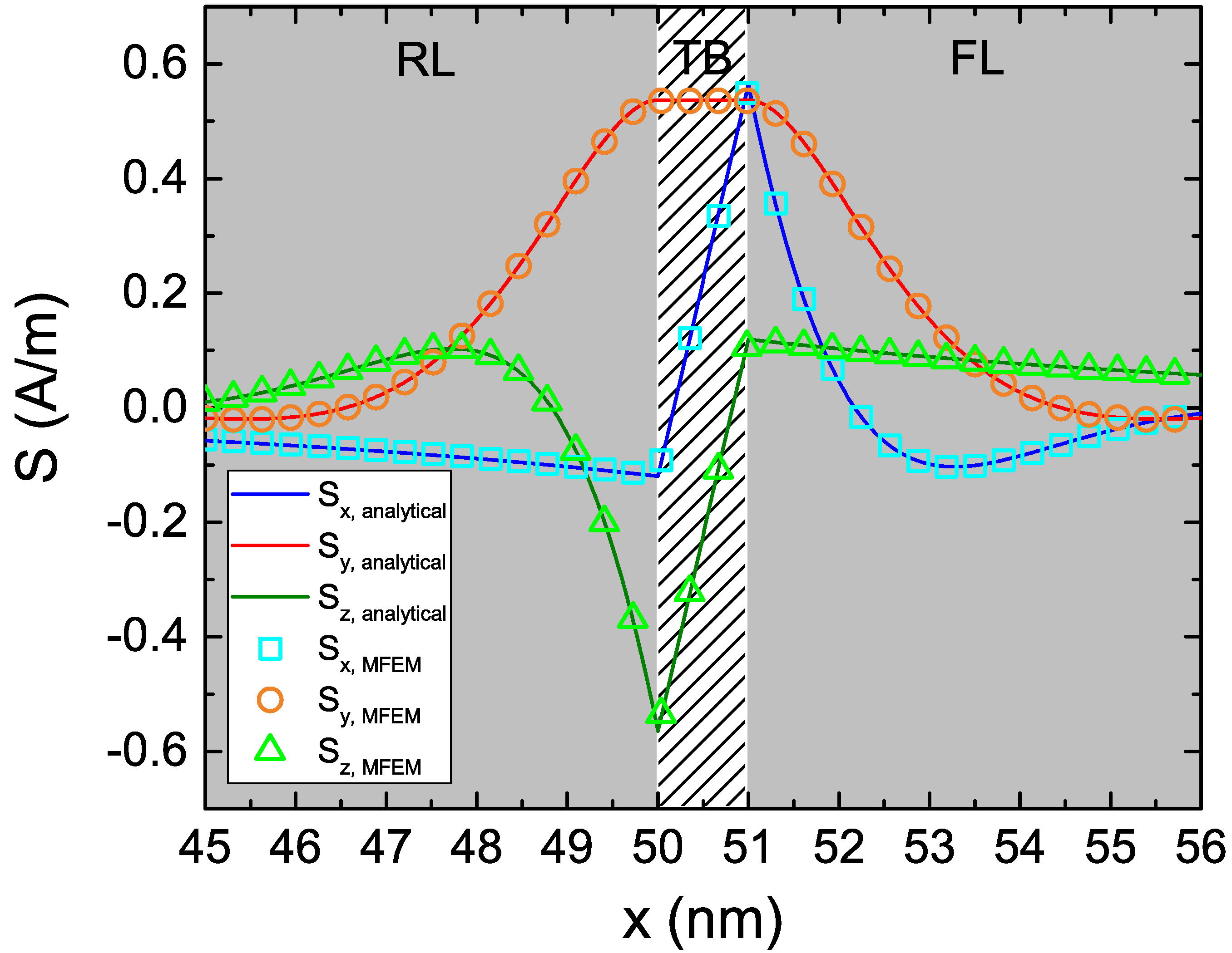
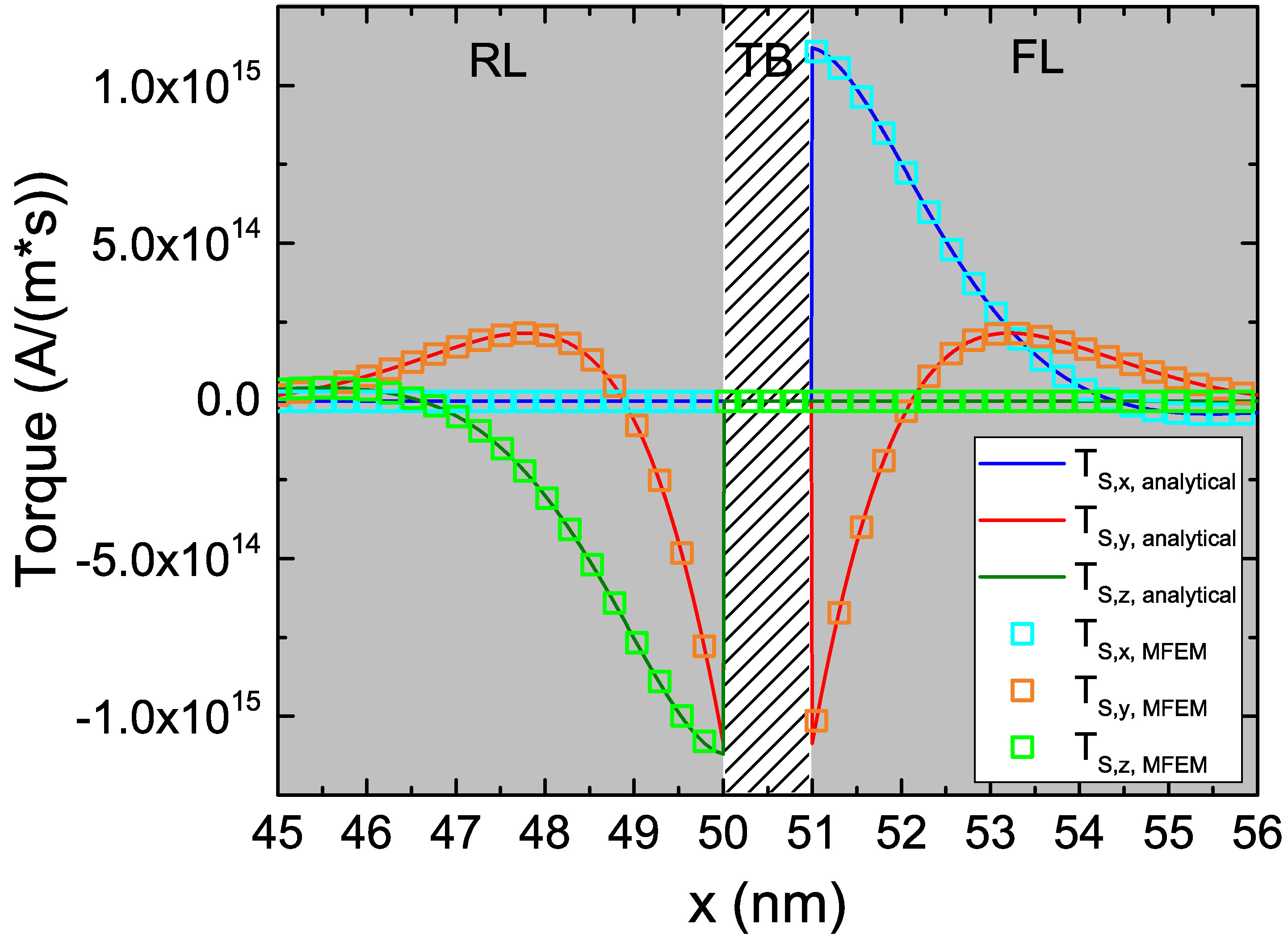
Figure 8.1: Spin accumulation (a) and torque (b) computed with the inclusion of the tunneling spin current, for semi-infinite FM layers. The analytical solution is compared with the FE one, computed with the inclusion of the
spin-current boundary condition 8.2, showing perfect agreement. Magnetization is along in the RL, along in the FL.
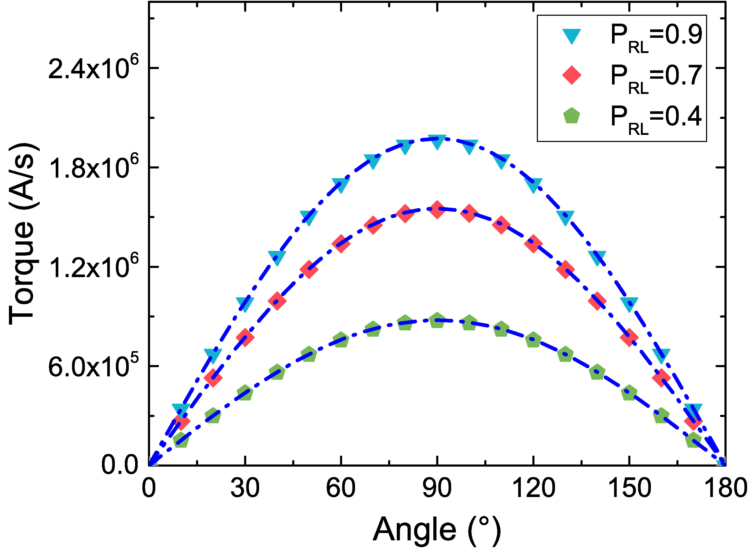
Figure 8.2: Angular dependence of the torque with the spin-current boundary conditions, for semi-infinite FL and RL. The expected sinusoidal angular dependence of an MTJ is reproduced, for several values of the RL spin polarization
parameter. The figure was adapted from [13].
8.1.1 Spin Accumulation and Spin Torque Solutions
In Fig. 8.1, the spin accumulation and torque obtained from the parameters of Table 8.1 are reported. The structure employed has
semi-infinite ferromagnetic leads and TB of 1 nm thickness. The magnetization of the RL points in the x-direction, while the one of the FL points in the z-direction. The FE solution is compared to the analytical one, showing
that the additional boundary terms in the FE implementation are able to create perfect agreement between the two. The inclusion of the tunneling spin current terms creates a jump between the values of the spin accumulation
components parallel to the magnetization at the left and right interface of the TB. This is the manifestation of the MTJ polarization effects on the spin current [166].
Fig. 8.2 shows the angular dependence of the damping-like torque with the inclusion of the spin current boundary conditions, computed in the same structure through (7.4) without the division by the FL thickness. The typical simple sinusoidal dependence [16], [99], [118] of the torque acting on the FL in an MTJ is now reproduced exactly, for various values of the RL|TB interface
spin polarization. The structure is biased by a fixed voltage of V, so that the torque is independent of the TB|FL polarization, and only depends linearly on the value of the RL|TB one.
(a)
(b)
(c)
(d)
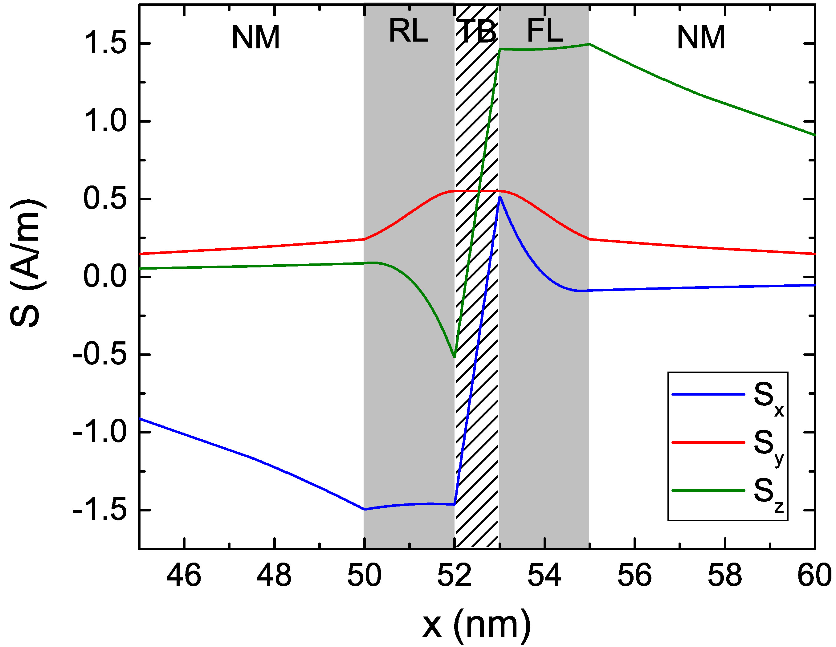
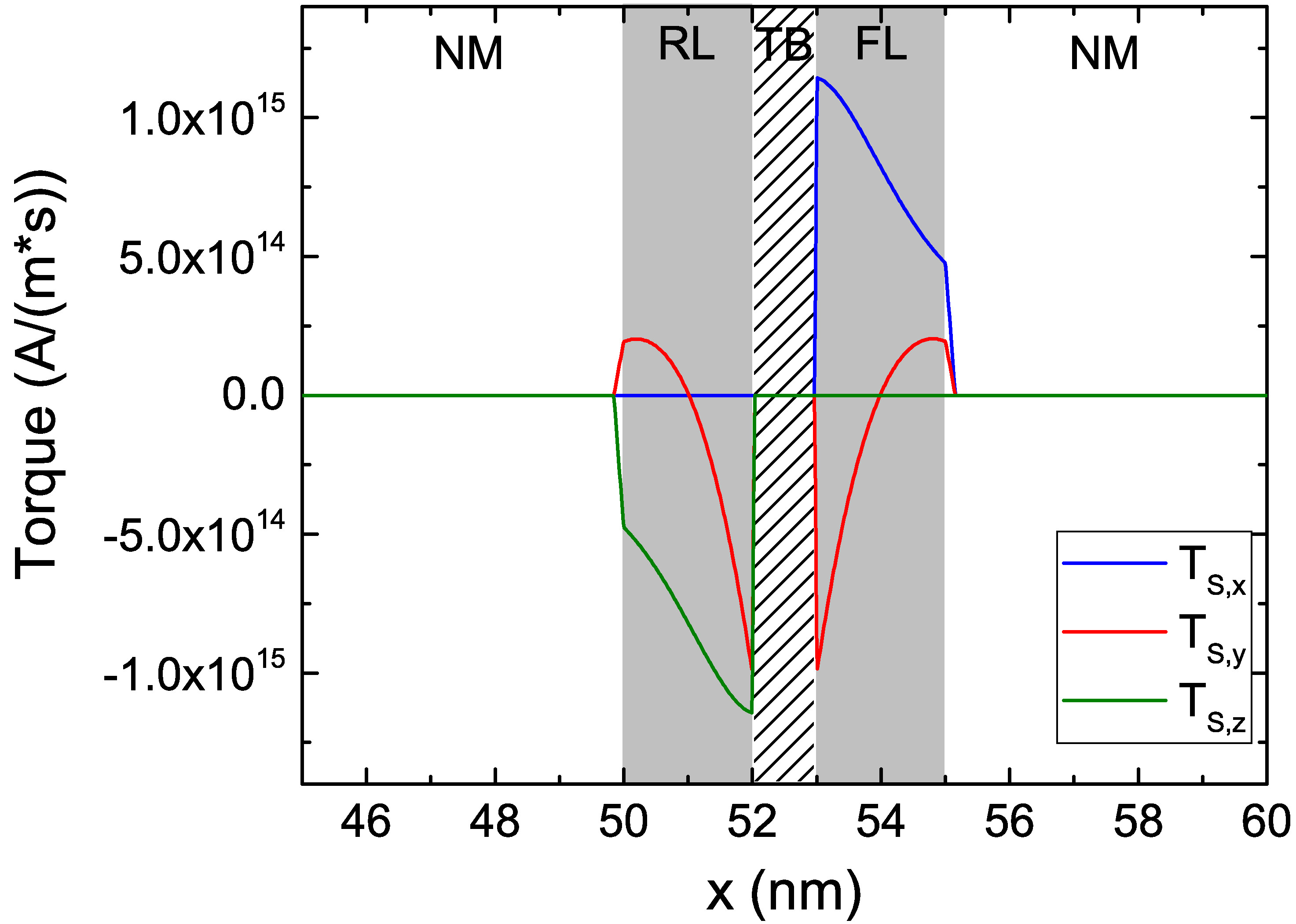
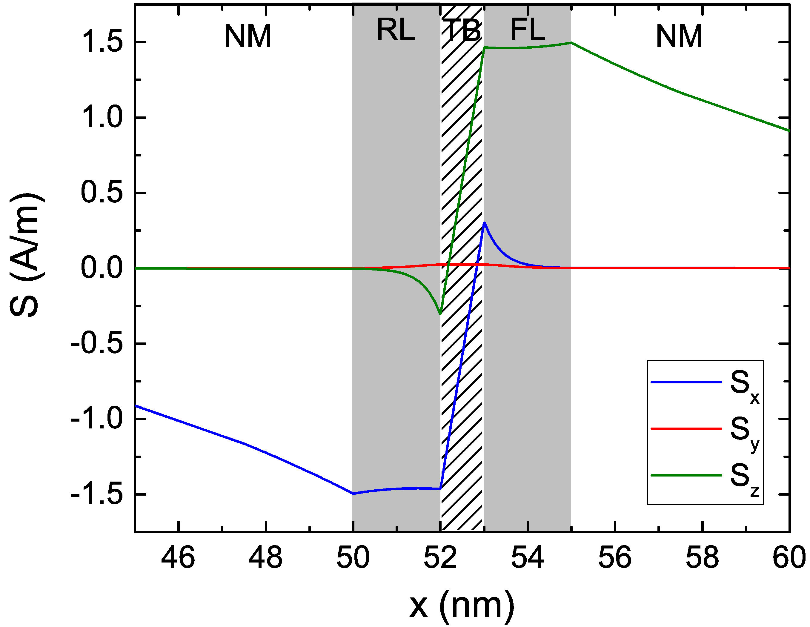
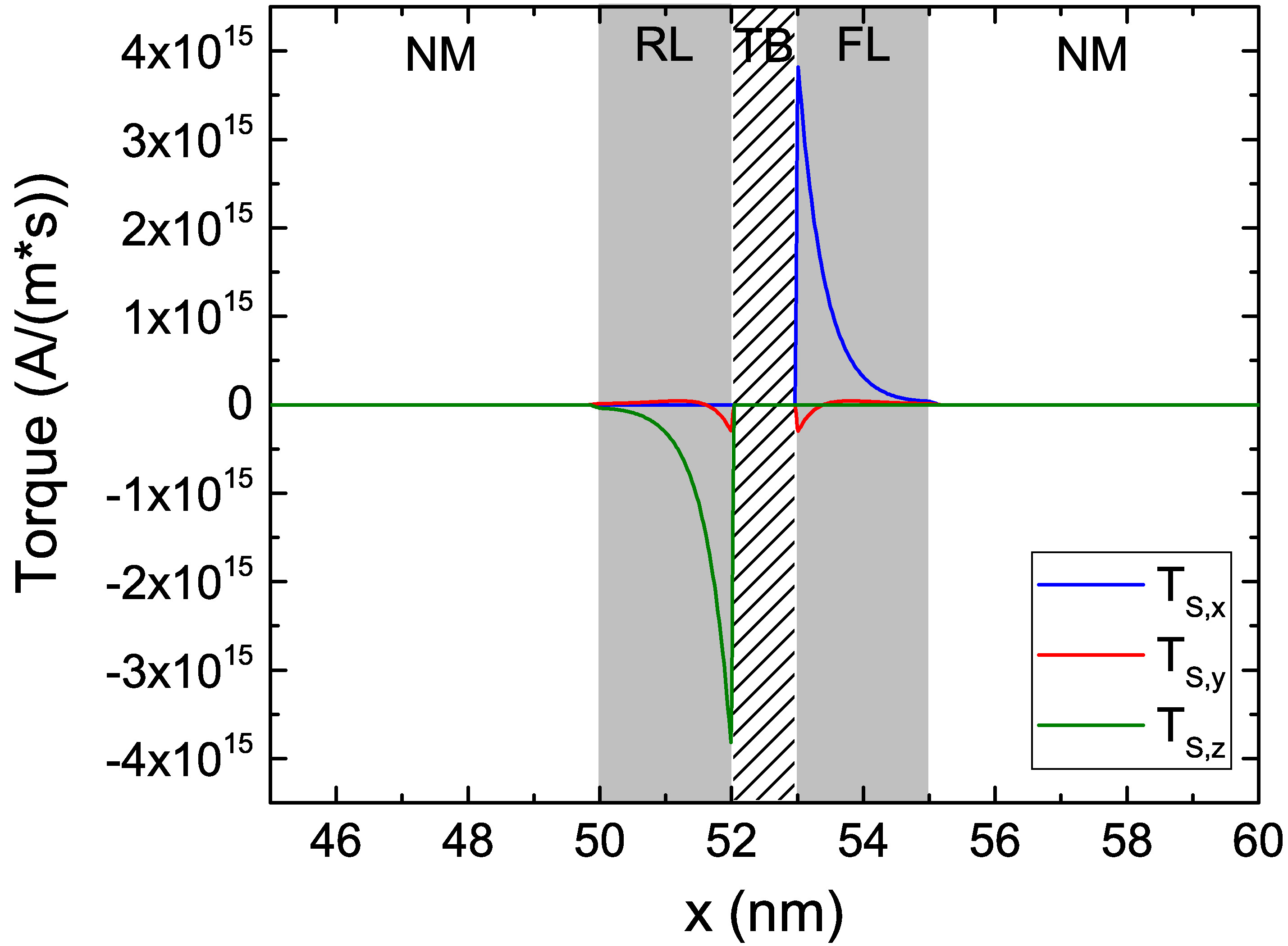
Figure 8.3: Spin accumulation and torque in a symmetric MTJ structure including NM contacts. (a) and (b) present results for nm. (c) and (d) present results for nm. (a) and (c) were adapted from [164].
While employing (8.2) gives the opportunity to fix the spin current in the TB to the value expected in MTJs, the length parameters entering (6.38) still determine the region over witch the transverse spin accumulation components are absorbed and the behavior of the torque in the bulk of the FM
layers. Fig. 8.3(a) and Fig. 8.3(b) show the spin accumulation and torque obtained in a symmetrical MTJ
structure including 50 nm thick NM layers, where the FM layers are 2 nm thick and the TB is 1 nm thick. The material parameters and magnetization orientation are the same as the ones employed for
Fig. 8.1. In this case, the torque components are not completely absorbed in the FL, contrary to what is usually expected in strong ferromagnets [16], [155], and the spin accumulation components transverse to the local magnetization penetrate inside the NM
contacts. By taking an effective dephasing length of nm, it is possible to guarantee a faster decay of the transverse spin accumulation components [120], so that the torque acts only in the proximity of the TB interface (cf. Fig. 8.3(c) and Fig. 8.3(d)).
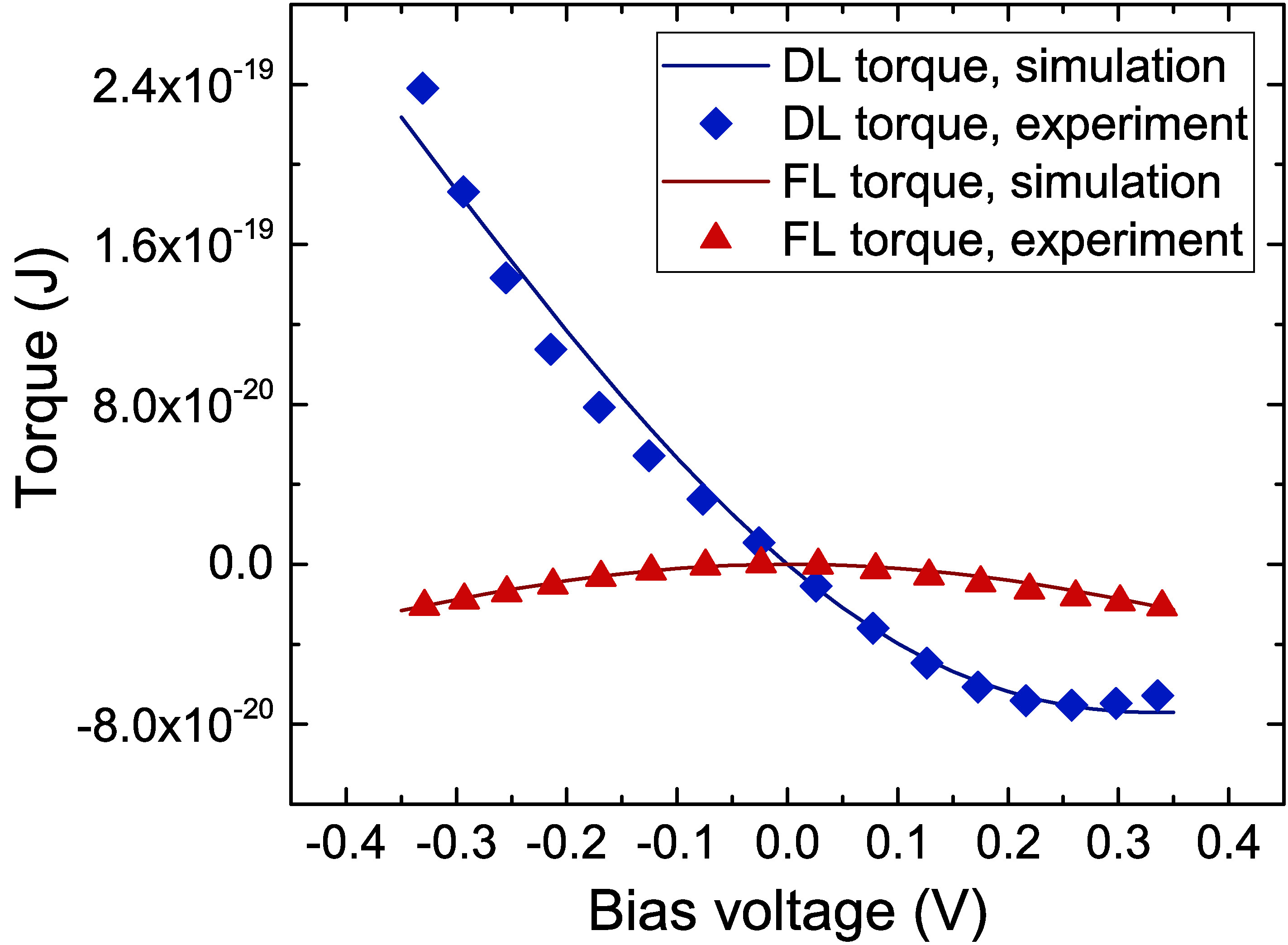
8.1.2 Voltage Dependence of the Spin Torques and TMR
(a)
(b)
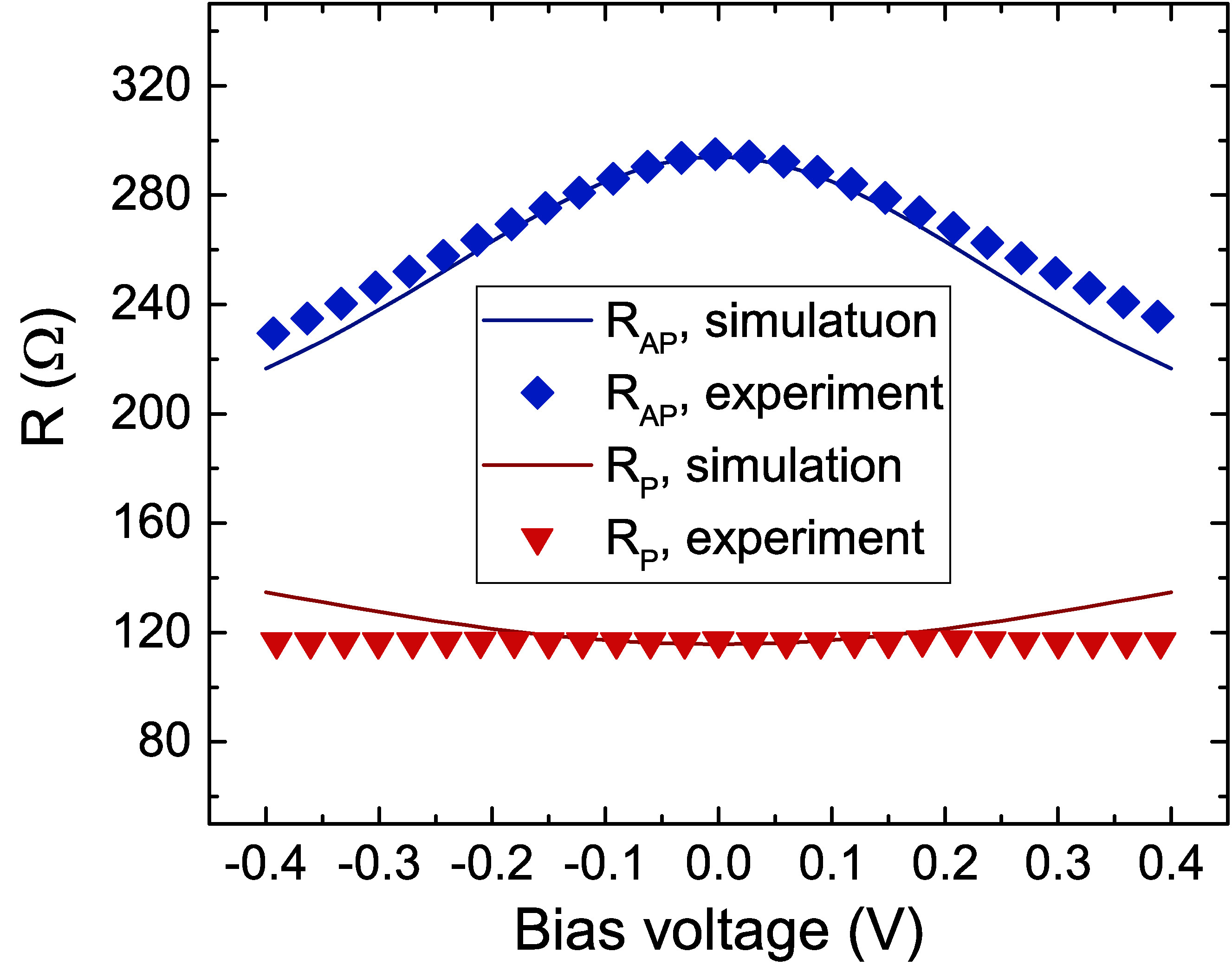
Figure 8.4: Dependence of both resistance (a) and damping-like (DL) and field-like (FL) torques (b) on the applied bias voltage, compared with the experimental results from [159].
Table 8.2: Parameters employed for reproducing the experimental results from [159].
.
Parameter
Value
Zero bias polarization,
TB conductance,
S
In-plane torque reduction,
Out-of-plane polarization,
Voltage dependence strength,
0.65 V
The implementation discussed until now still produces a linear dependence of the torques on the bias voltage, with a vanishing field-like component for . As already mentioned at the end of Chapter
7, fabricated MRAM devices usually exhibit clear non-linearity in the observed voltage dependence of the torques, with the TMR value also depending on the applied bias [159]–[162]. The presented approach gives the opportunity to account for this
non-linearity by having the polarization parameters and depend on the bias voltage. A phenomenological voltage-dependent expression can be postulated as [167]
Here, can be extracted from the TMR at zero bias TMR, and from the high bias behavior. A comparison of both TMR and torque results with experimental ones [159] is reported in Fig. 8.4. The values for the torque were obtained by integrating the torque over the whole FL volume, and
multiplying the result by . The parameters employed to fit the observed TMR and torque dependence on the bias voltage are reported in Table 8.2.
was extracted from the anti-parallel resistance and TMR=154% of the experimental structure, possessing a surface area of 70 nm250 nm. The
thicknesses of the RL, FL and TB are 3 nm, 2 nm and 1 nm, respectively. The torque and TMR obtained form the simulations show a good agreement with the experimental ones. A slight deviation of the
computed resistance from the experimental one can be observed at higher values of the applied bias. This discrepancy can be attributed to the constant value employed for the conductance [154]. The inclusion of a voltage dependent expression for the tunneling conductance [65] will provide a way to obtain an even
better fit to the experimental data.
8.2 GMR Effect in Spin-Valves
The approach detailed in the previous section is able to compute both the TMR and torques in an MTJ. Modern MRAM devices can however include also conductive spacer layers between the FM ones, either as part of the SAF [73], or to include additional RLs and improve the switching performance [168]. In the presence of such a metallic spacer layer,
the GMR effect can be of significance. In the drift-diffusion formalism, the resistance dependence on the relative angle between the magnetization vectors in the presence of a metallic spacer can be accounted for by including the
second right-hand side term of (6.7a) when computing the electrical potential . By taking (in the absence
of current sources, see (6.36c)) and expressing the electric field as in (6.7a), the equation for results in
The weak formulation of (8.4), including the computation of the electric field and charge current density from , becomes then
As the spin-dependent term in (6.7a) is already taken into account in the computation of , the spin current is described by
(6.7b). The weak formulation of the spin accumulation equation (6.38a), with the inclusion of the TB boundary terms, if one is present, can then be expressed as
In this formulation, the spin accumulation and the electrical potential depend on each other, creating a coupled system of equations. In order to take the interdependence of and into account, the FE solver is
updated to iterate over the solution of (8.5a) and (8.6) until a convergence threshold is reached. This approach can be directly applied to the FE implementation of the two separate equations, and does not require
additional care for the inclusion of the boundary condition (8.2) when solving a fully coupled system. The iterative solution is computed as follows:
1. A first estimate for the spin accumulation is obtained by solving (6.59) and (6.60) as before, with the right-hand side term of (6.7a) included in the spin equation
3. This solution is then used to obtain an updated spin accumulation estimate from (8.6)
4. Steps 2 and 3 are iterated until the solver reaches convergence
(a)
(b)
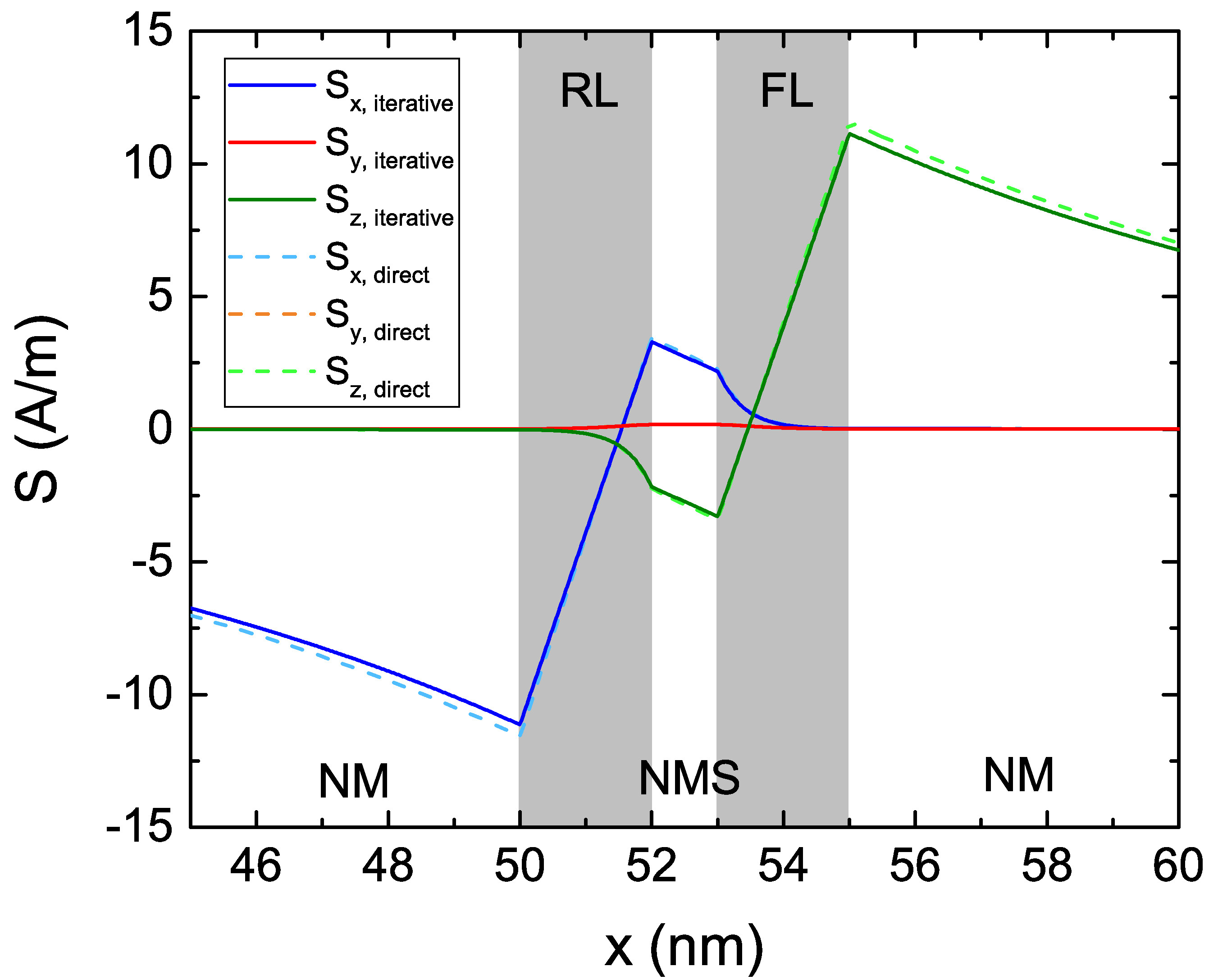
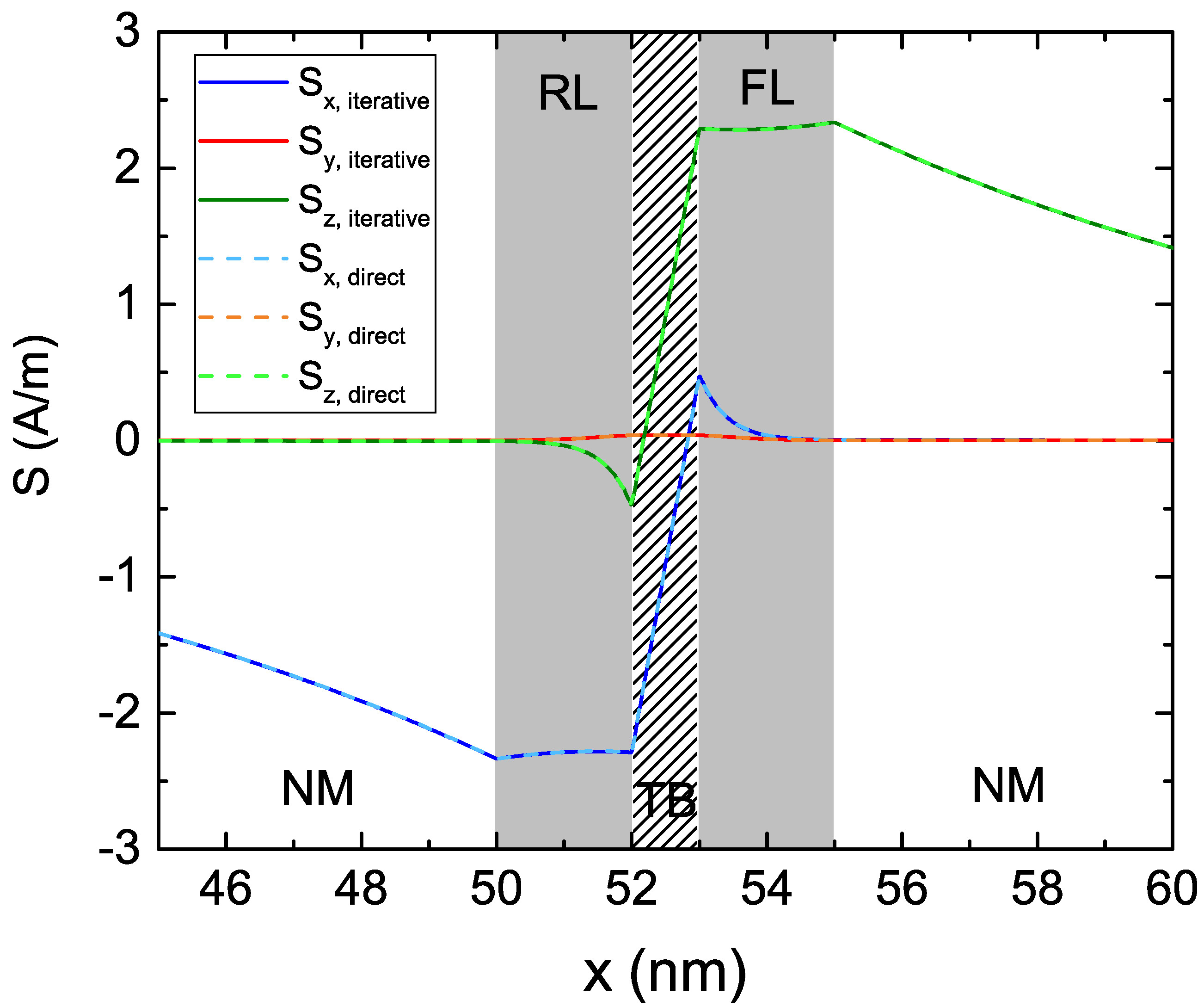
Figure 8.5: Comparison of the solution of the iterative method described in this section to the one obtained by solving (6.59) and (6.60), for both a spin-valve (a) and an MTJ (b).
(a)
(b)
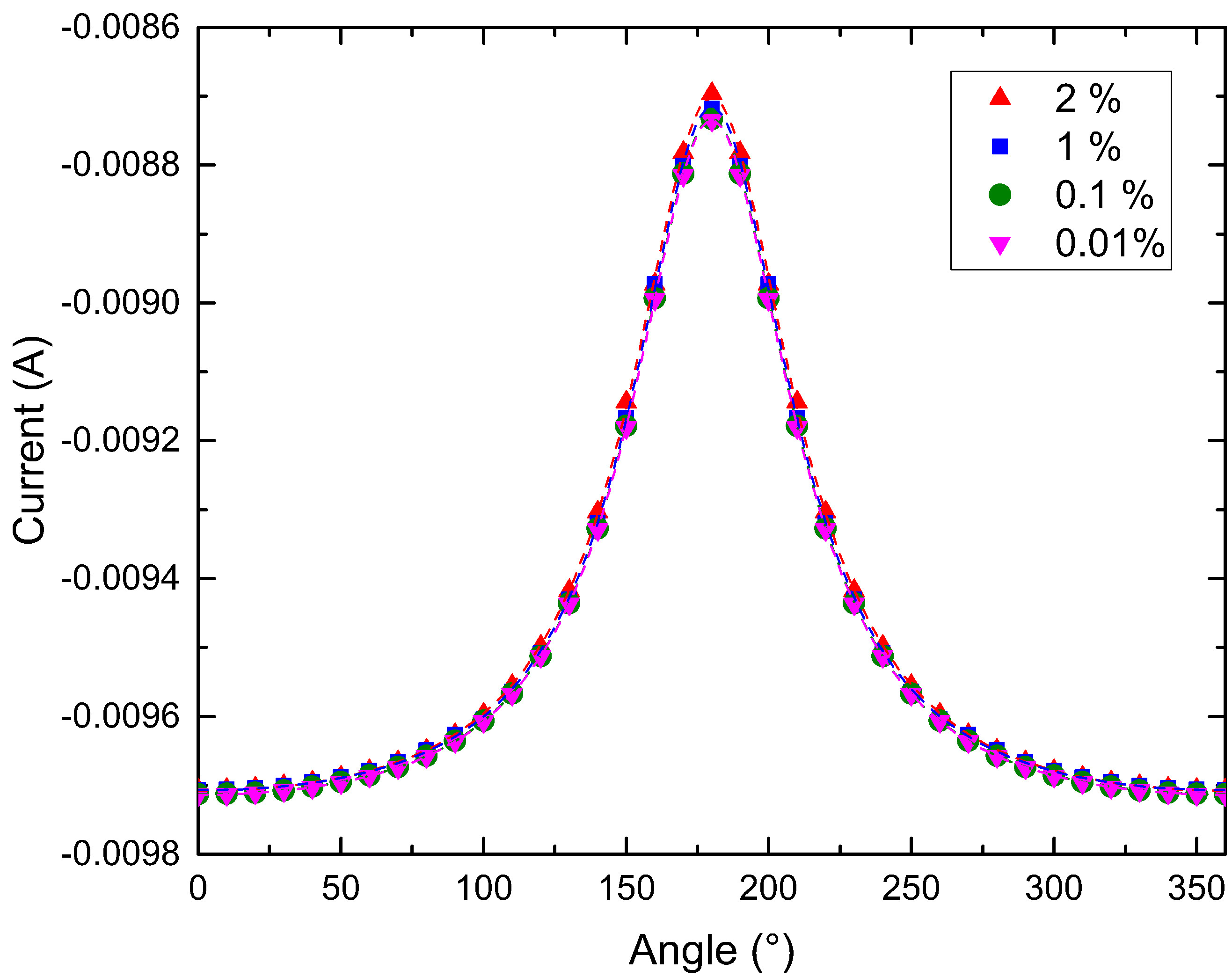
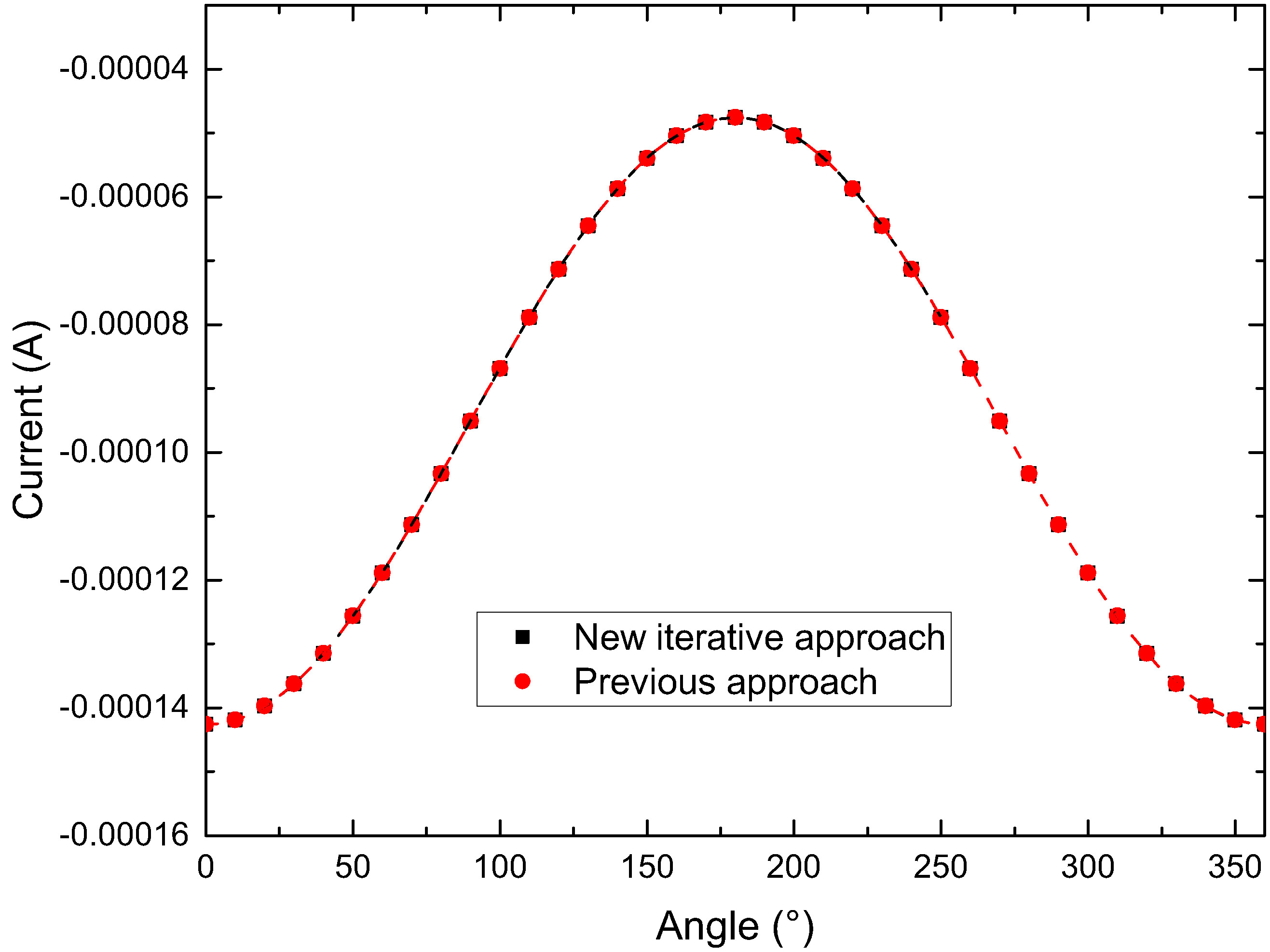
Figure 8.6: (a) Angular dependence of the total charge current in a spin-valve structure with metallic spacer, computed with the iterative approach for various values of the convergence parameter . (b) Angular
dependence of the torque in an MTJ, computed using both the direct and iterative approach. The figures were published in [13].
In Fig. 8.5(a), the spin accumulation solution in a spin-valve obtained from the iterative approach is compared to the one computed using (6.59) and (6.60). The structure has the same dimensions as the one employed for the results
presented in Fig. 8.3, with an NMS in place of the TB. The parameters are the ones of Table 8.1, with nm. The two solutions show only a marginal difference between each other, testifying the fact that the iterative approach is useful in case one is interested in the GMR effect, but can be avoided if the main focus is on
the computation of the torque and magnetization dynamics. In Fig. 8.5(b), the same comparison is shown for the solution in an MTJ, with a TB separating the two FM layers.
In this case, the two solutions show perfect agreement between each other.
Fig. 8.6(a) shows the obtained dependence of the total charge current on the relative angle between the magnetization vectors in the FL and RL, for several values of .
The solution is computed in the structure in Fig. 1.1, with the middle layer treated as an NMS, for an applied voltage of V. The dashed lines represent a fit carried out
using the equation [169]
where is the applied bias voltage, is the resistance in the parallel state, and and GMR are used as fitting parameters. The GMR value is , with the results obtained using
converging fast () and giving a good approximation.
As the voltage drop is localized at the TB in an MTJ, the iterative solution is not necessary for the correct computation of the current. In order to confirm this, the charge current angular dependence with a tunneling middle layer
is computed both by using the direct solution of equations (6.59) and (6.60), and by employing the iterative solution described in this section. The obtained results are reported in Fig. 8.6(b). The
fitting can be performed by using the angular dependence expression (7.1). As the iterative solver always converges for and the results
are indistinguishable from the direct solution, these findings confirm that the latter can be safely employed for all structures only containing MTJs.
8.3 Torques in Elongated Ultra-Scaled Devices
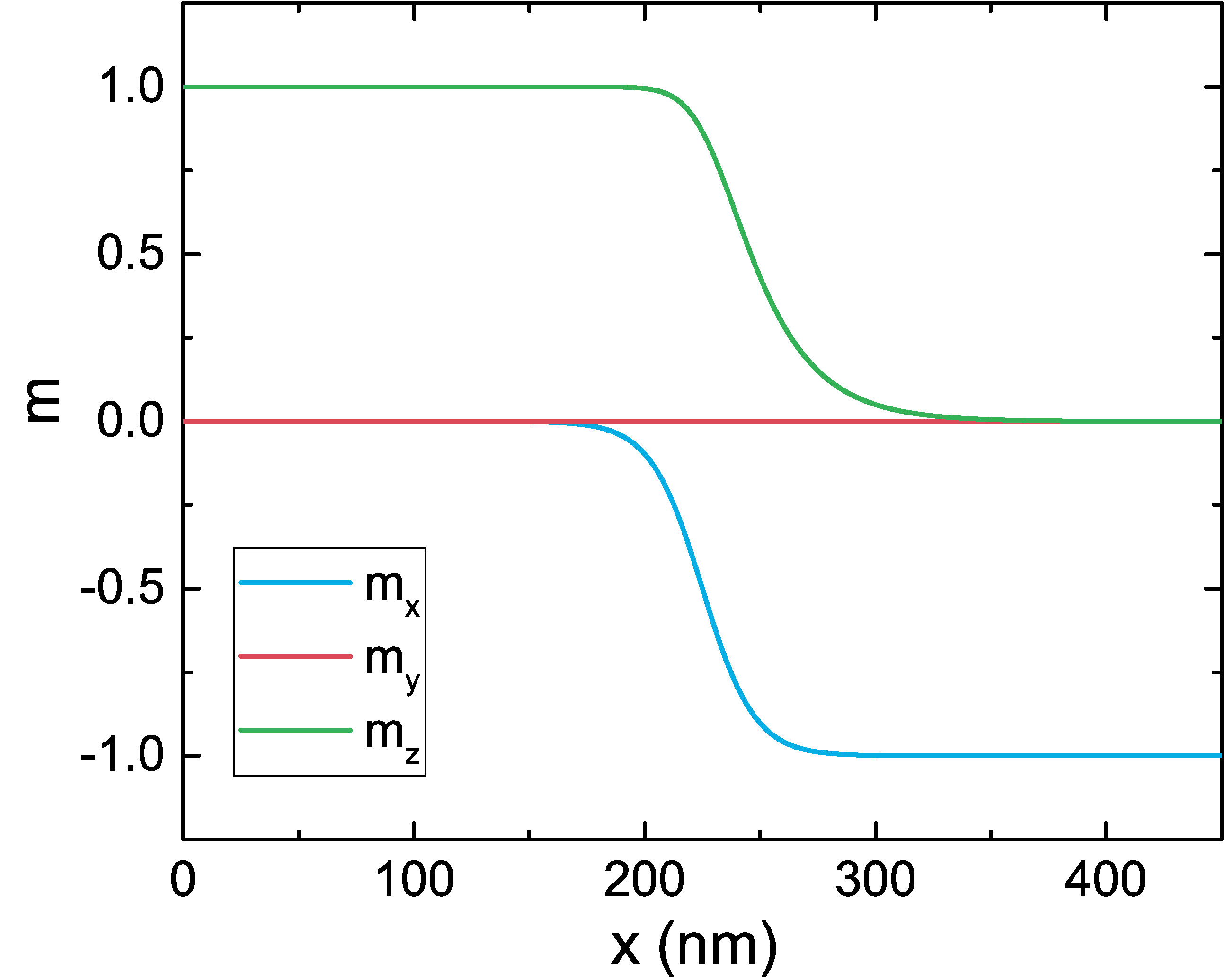
(a)
(b)
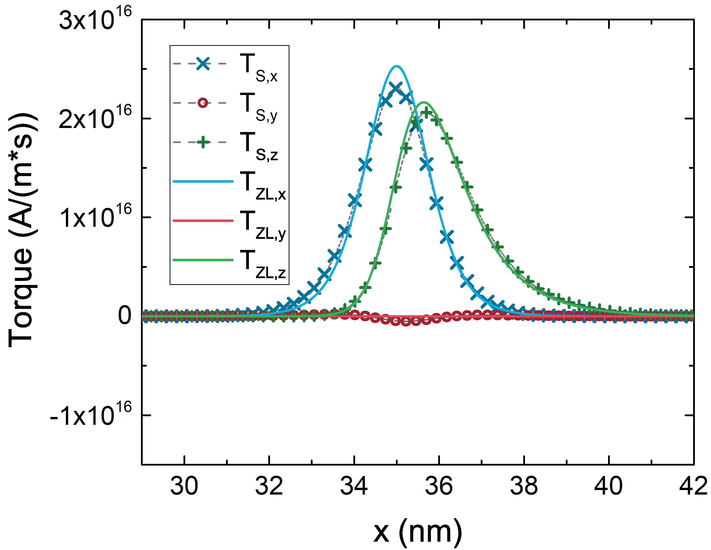
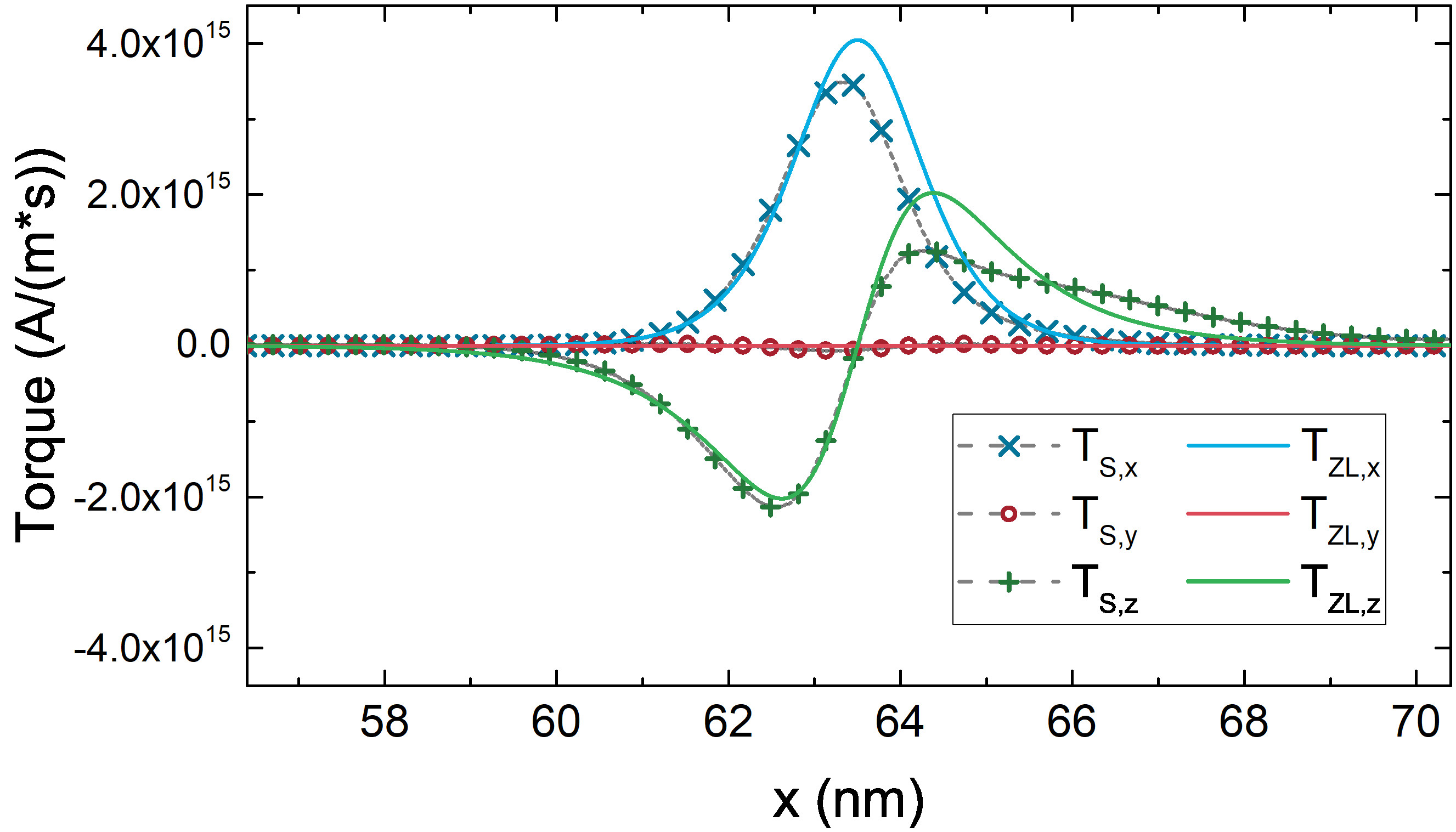
Figure 8.7: (a) Non-uniform magnetization texture with the magnetization orientation changing from z to -x. (b) Comparison of the spin torque to the Zhang-Li torque for a
nm long magnetization texture, with the parameters of Table 8.1. The two approaches are in good agreement. The figures were adapted from [13].
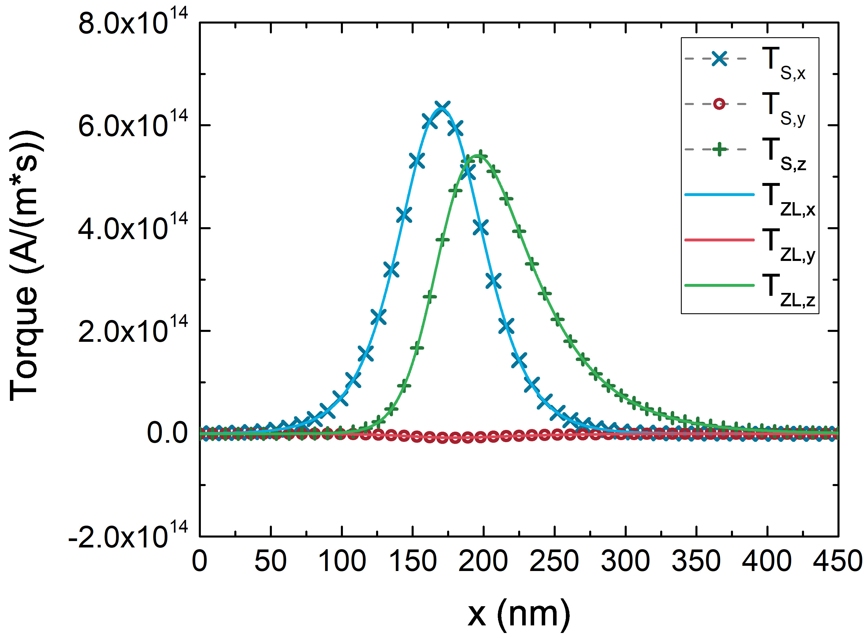
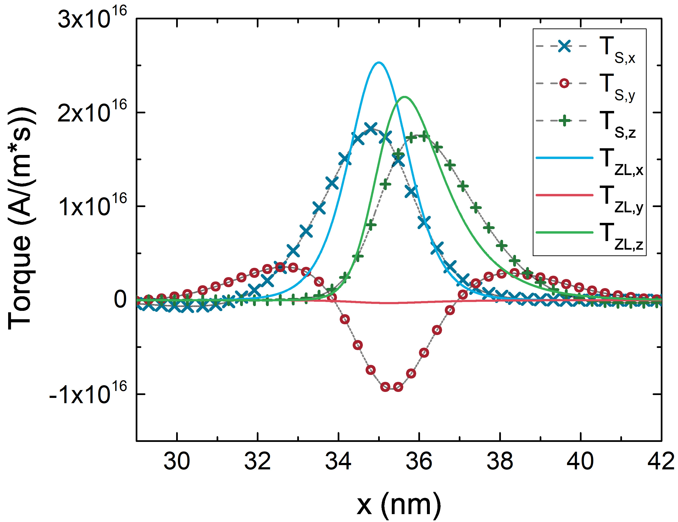
(a)
(b)
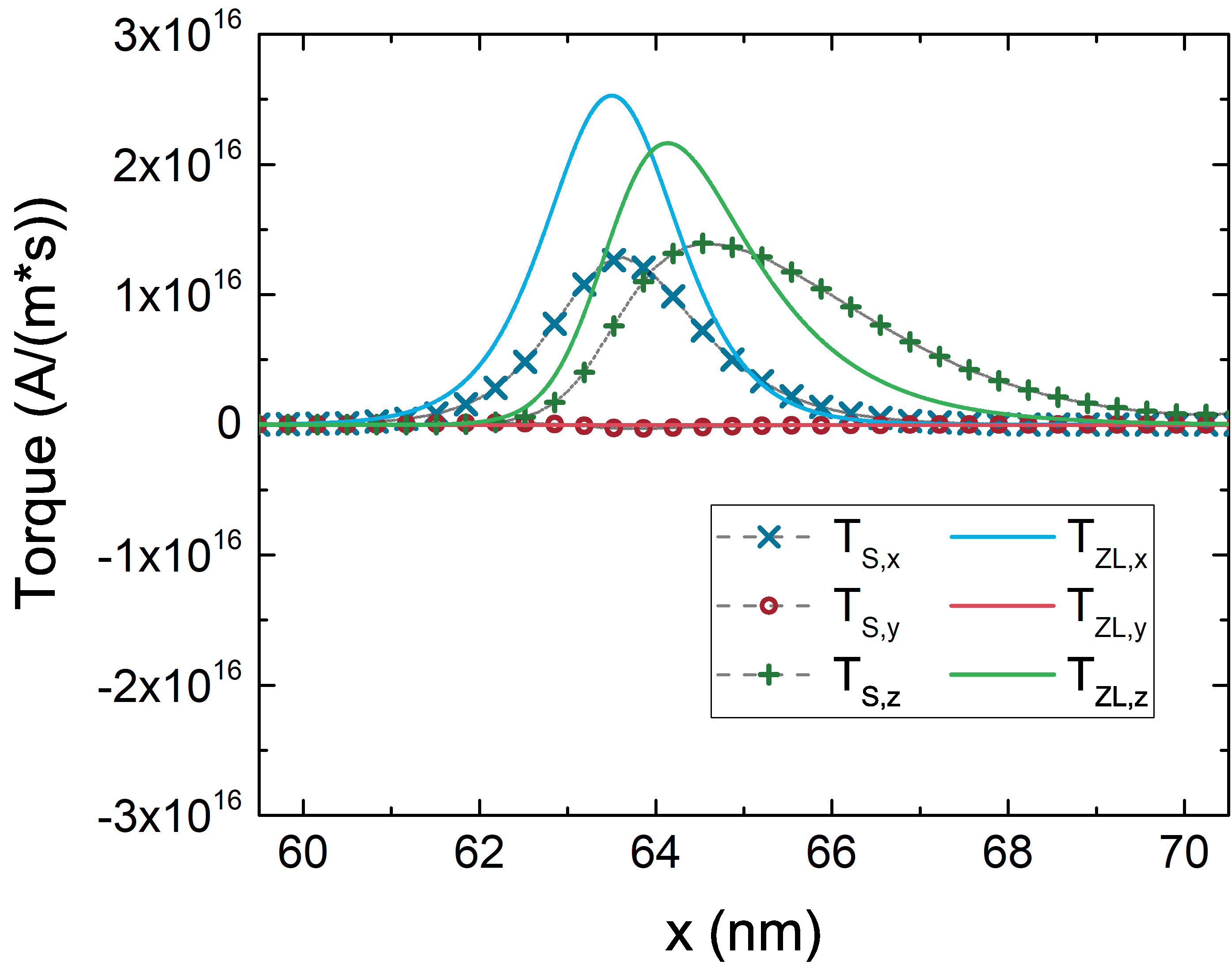
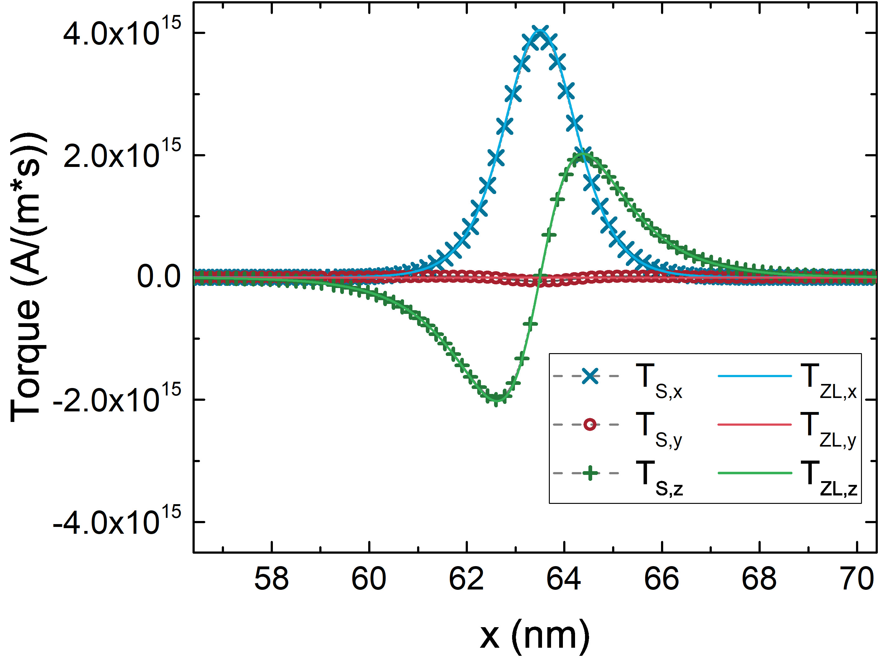
Figure 8.8: Comparison of the spin torque to the Zhang-Li torque for a a nm long magnetization texture, for the parameters of Table 8.1
in (a) and nm in (b). The shorter dephasing length takes the role of quickly absorbing the transverse spin accumulation components, so that the agreement between the ZL approximation and
the drift-diffusion solution is recovered. The figures were adapted from [13].
In the presence of elongated FLs like the ones in Fig. 1.2, the switching of the whole layer at the same time is not guaranteed: a domain wall or magnetization textures can be
generated, with their propagation through the FL affecting the switching behavior. In this case, the additional spin torques created by the presence of magnetization gradients in the bulk of the ferromagnetic layers must be taken
into account. These torques are modeled by the Zhang and Li (ZL) equation [151]
where . This expression can be obtained from (6.12) by taking
and cross-multiplying two times by . This approximation is strictly valid only when the changes in are relatively slow, namely, when they happen over length
scales longer than . By applying the same procedure to (6.38), (8.9) can be generalized to include , obtaining the following expression:
accounts for the additional contributions of the term involving .
In order to test the ZL approximation, the magnetization profile shown in Fig. 8.7(a) is employed to compute both and ,
with the parameters of Table 8.1. The structure used for the simulations is a single ferromagnetic layer of 450 nm. The same constant current density value of A/m, flowing in the x-direction, is employed for the two approaches. Fig. 8.7(b) demonstrates that, for the given magnetization
profile, with width of nm, is well reproduced with (8.9).
Fig. 8.8(a) reports the torques obtained by using the same parameters and a shorter magnetization texture of nm, in a FM layer of 70 nm thickness.
In this case, the spin accumulation gradients neglected in (8.9) affect the result, and a large deviation of from is
observed, especially for the field-like torque (y-component). However, when the effective short value of the spin dephasing length is employed, it guarantees the fast absorption of the transverse spin
accumulation components, and recovers a good agreement with , as shown in Fig. 8.8(b).
In MRAM cells with elongated FLs, magnetization textures and domain walls can form along the layer during switching. In this case, the polarized tunneling spin current can interact with such magnetization textures, and create
torques that further deviate from the ZL approximation. In order to verify this, the torque is computed in an experimental MTJ structure, reported in [22] and shown in the top
of Fig. 1.2. The cell employed for this simulations has a nm RL, nm TB (TB), and an elongated FL of nm with a magnetization
profile in the FL similar to the one shown in Fig. 8.7(a), with the magnetization vector going from the z-direction to the -x-direction over the length of the layer. The
magnetization in the RL is pointing towards the x-direction. The FL is additionally capped by a second 0.9 nm TB (TB), and 50 nm NM contacts are included. The solution is computed with the same
parameters as the ones employed for Fig. 8.8(b). The resistance of the overall cell in the parallel state and the polarization parameters used for the two TBs, extracted
from the data in [22], are reported in Table 8.3. All parameters pertaining each TB are taken to be equal between its left
and right interfaces. As the second TB is only added to grant an additional source of perpendicular anisotropy, thanks to the CoFeB|MgO interface, it can be fabricated to have minimal impact on the total resistance of the
structure [21]. For this reason, its conductance is taken to be 5 times greater than the one separating RL and FL. Moreover, as it is directly interfaced with the NM contact, it is
also taken to have a lower polarization than the main TB.
(a)
(b)
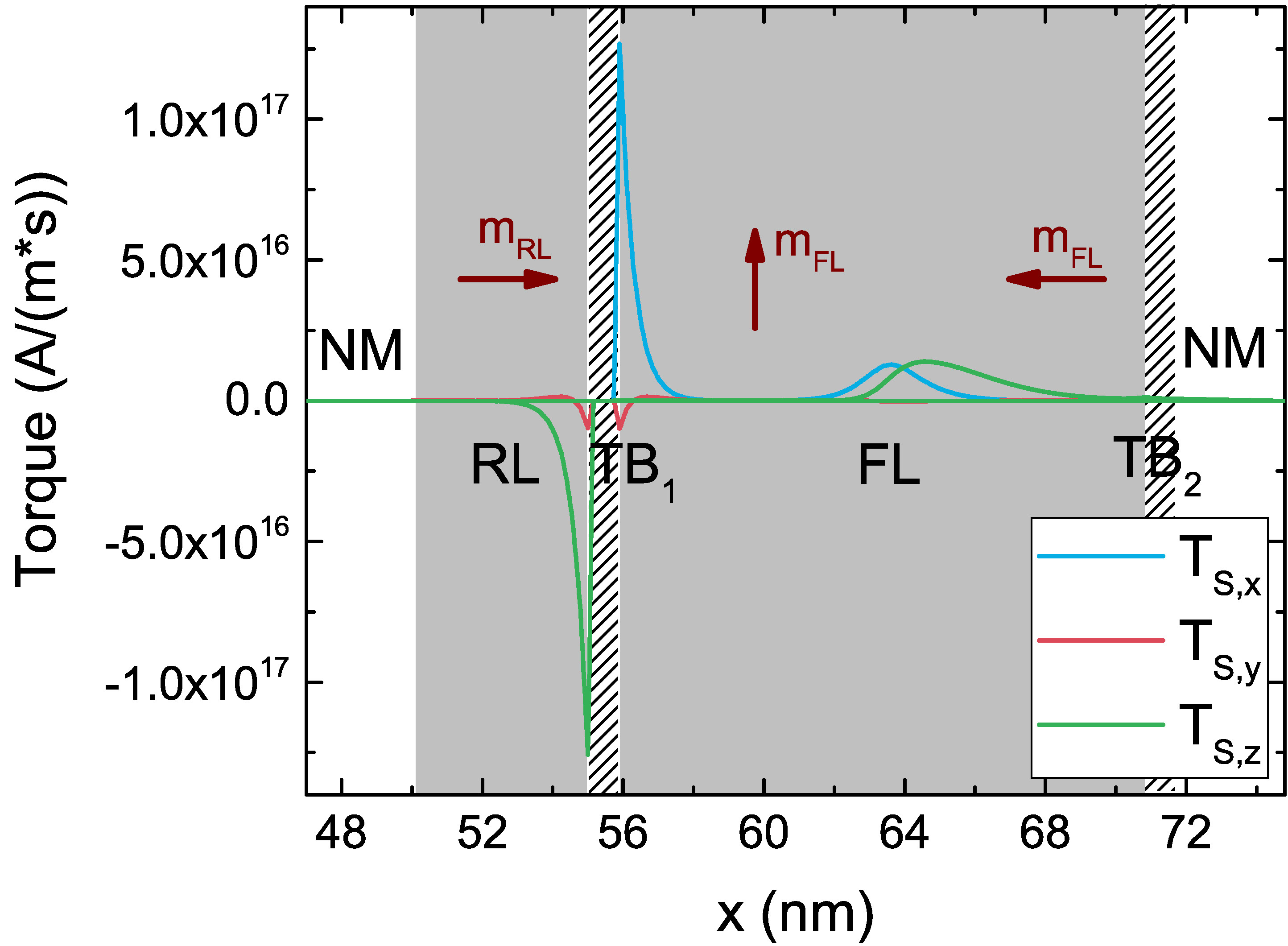
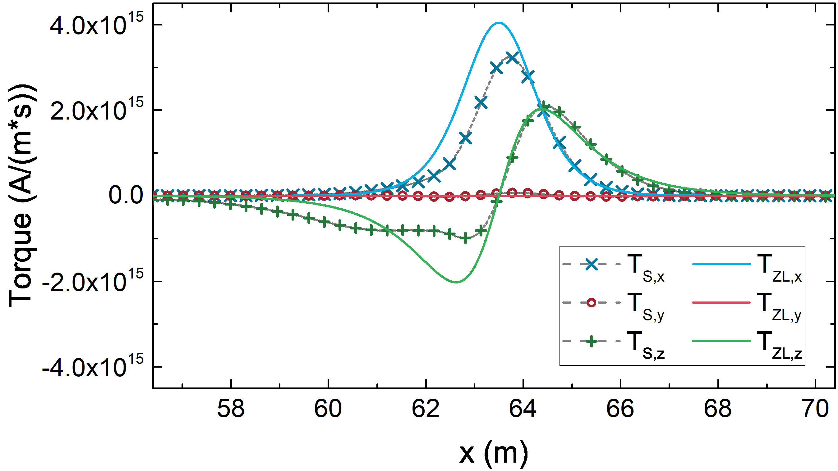
Figure 8.9: (a) Torque computed for an MRAM cell with elongated RL and FL and a magnetization profile in the FL similar to the one of Fig. 8.7(a), with a width of
nm. The brown vectors indicate the magnetization direction in the RL and in two parts of the FL. (b) Close-up of the spin torque compared to the Zhang-Li torque . The presence of the MTJ influences also the bulk portion of the torque, making the unified approach the most suitable for dealing with ultra-scaled MTJs with elongated ferromagnetic layers. The figures were adapted from
[13].
Table 8.3: Parameters used for the structure with elongated FL.
.
Parameter
Value
Parallel resistance,
k
TB polarization factor,
TB polarization factor,
The torque acting in the FL for this magnetization profile is shown in Fig. 8.9(a), where the magnetization vectors in each part of the FM layers
are also reported. Near the first TB, a Slonczewski torque contribution generated by the tunneling spin current can be observed, while the magnetization texture causes the torque contribution in the bulk. In Fig. 8.9(b) a close-up of the bulk portion of , compared with the result obtained by applying the ZL expression (8.10) to the magnetization configuration of the FL, is reported, for the same value of the current density. The comparison reveals a substantial difference between the torques obtained with
the presented model and the ZL approximation, even for the short value. This implies that the Slonczewski and ZL torque contributions cannot simply be added together, but influence and interact
between each other.
(a)
(b)
Figure 8.10: (a) Torque computed in a single FM layer with the magnetization going from the x- to the -x-direction over a domain wall of nm. The ZL expression produces a torque in perfect agreement with the
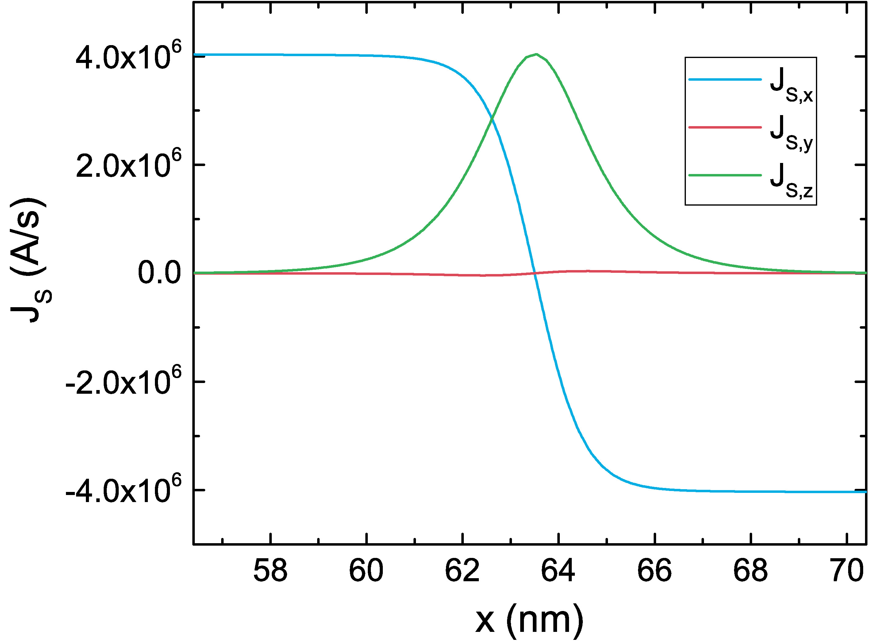
drift-diffusion one. (b) Spin current flowing in the x-direction, computed from the drift-diffusion solution. The three components follow the magnetization profile.
In order to further elaborate on how the presence of the TBs influences the torque generated by the magnetization texture, the drift-diffusion solution is computed and compared to the ZL one with different values of the
polarization parameter of the second barrier, . The magnetization texture employed for the following results is a full domain wall, with rotating from +x to -x in the xz-plane. The value of the
current density, flowing in the x-direction, is A/m. First, the purely bulk solution, computed in a single FM layer, is reported in Fig. 8.10(a). The drift-diffusion and the ZL torques are in this case in perfect agreement. The three components of the spin current flowing in the x-direction, obtained from , are
reported in Fig. 8.10(b). The spin current follows the magnetization profile, with the x-component assuming the values of and on the left and right of the domain wall, respectively, dictated by the first term of (6.38b).
(a)
(b)
(c)
(d)
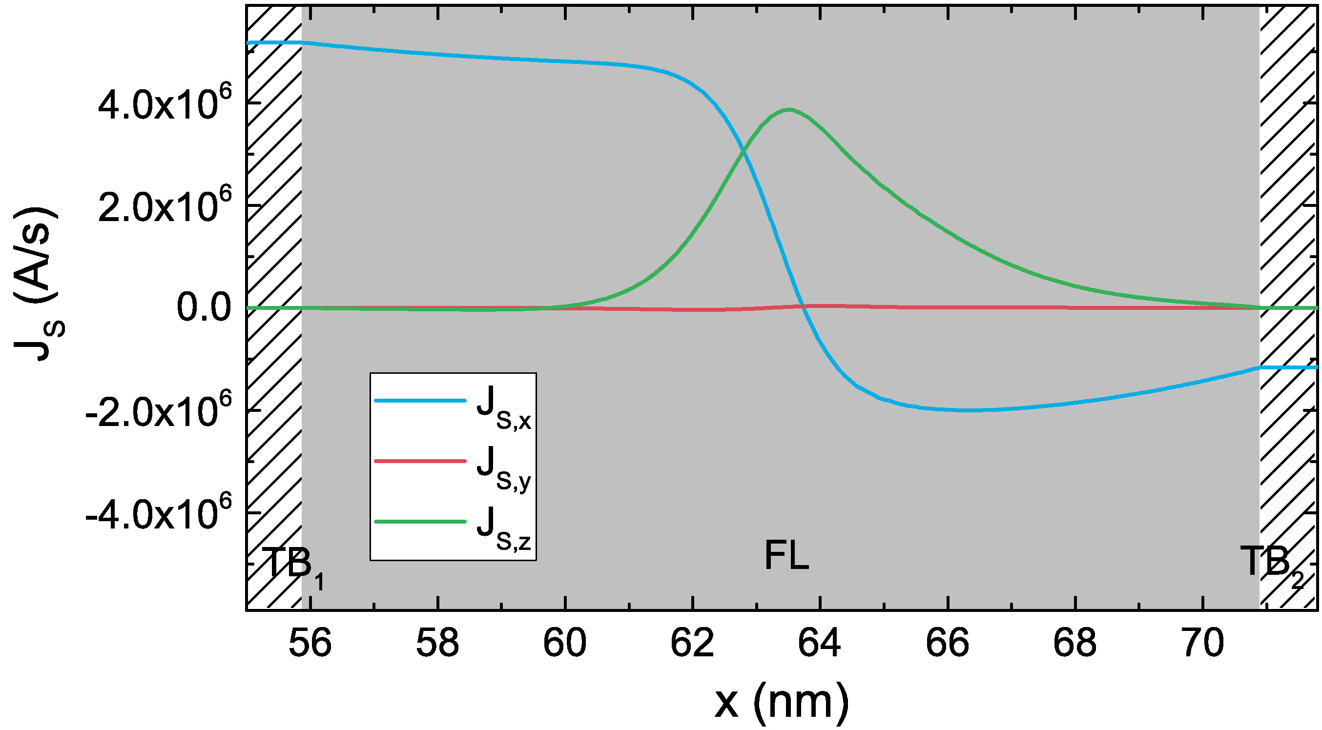
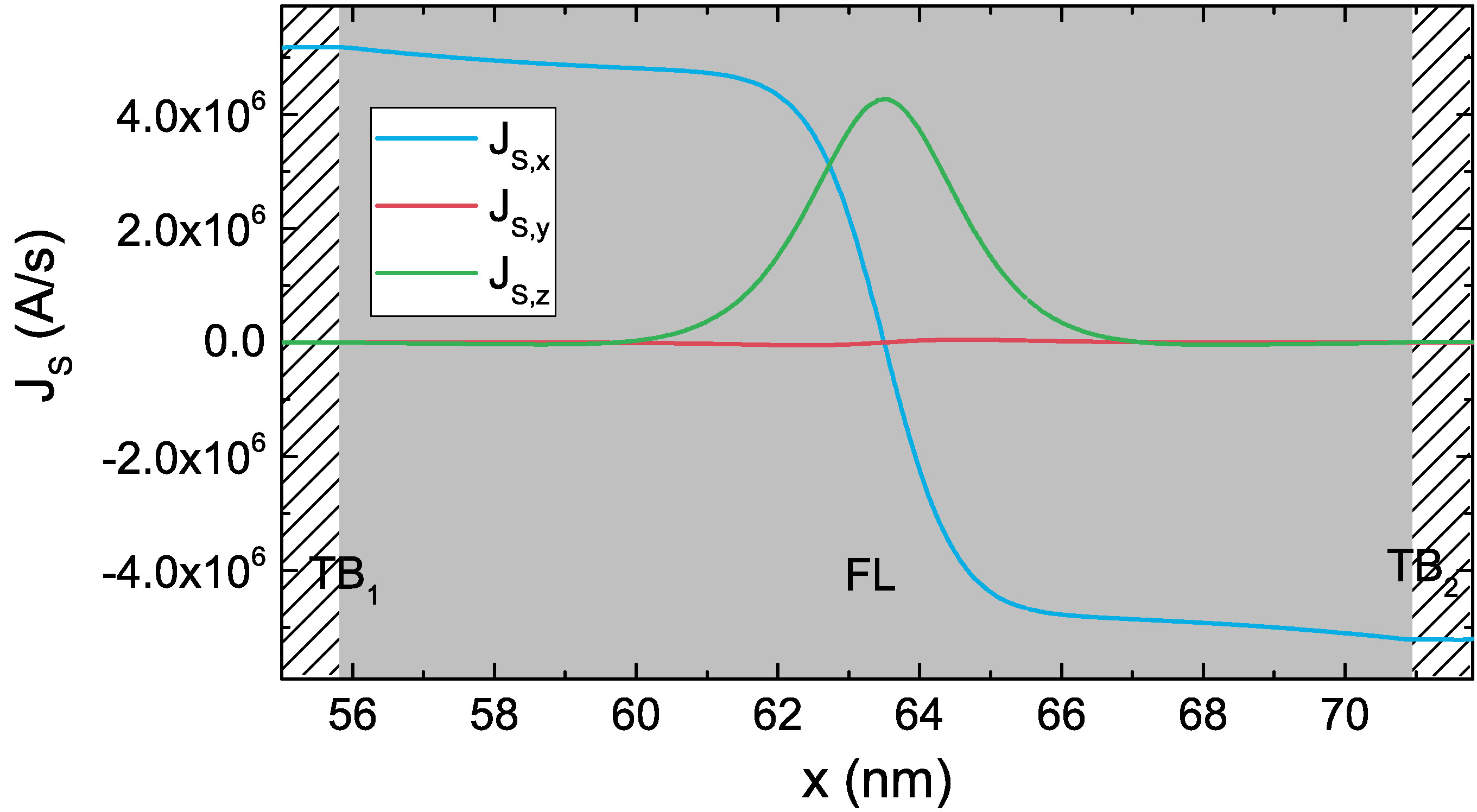
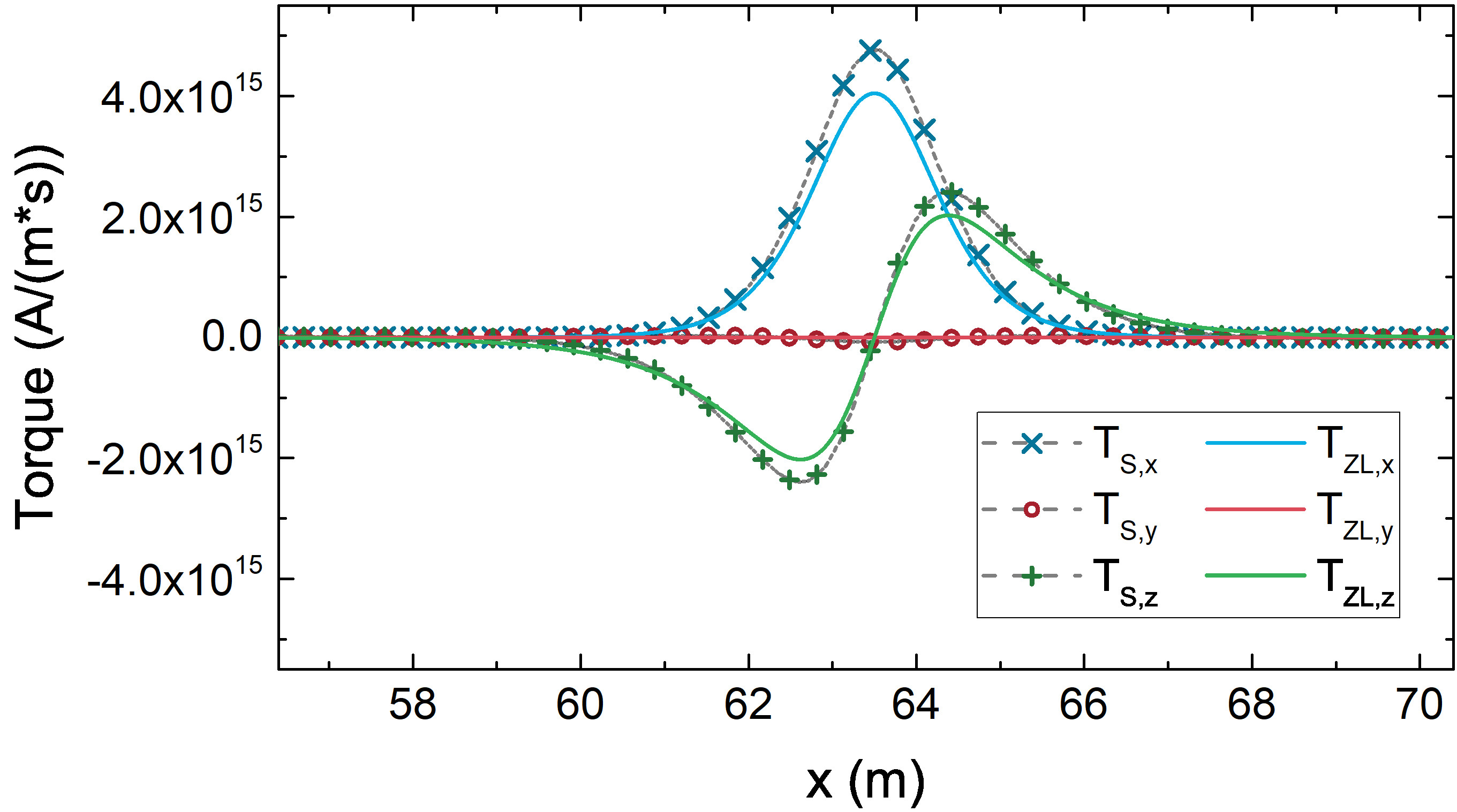
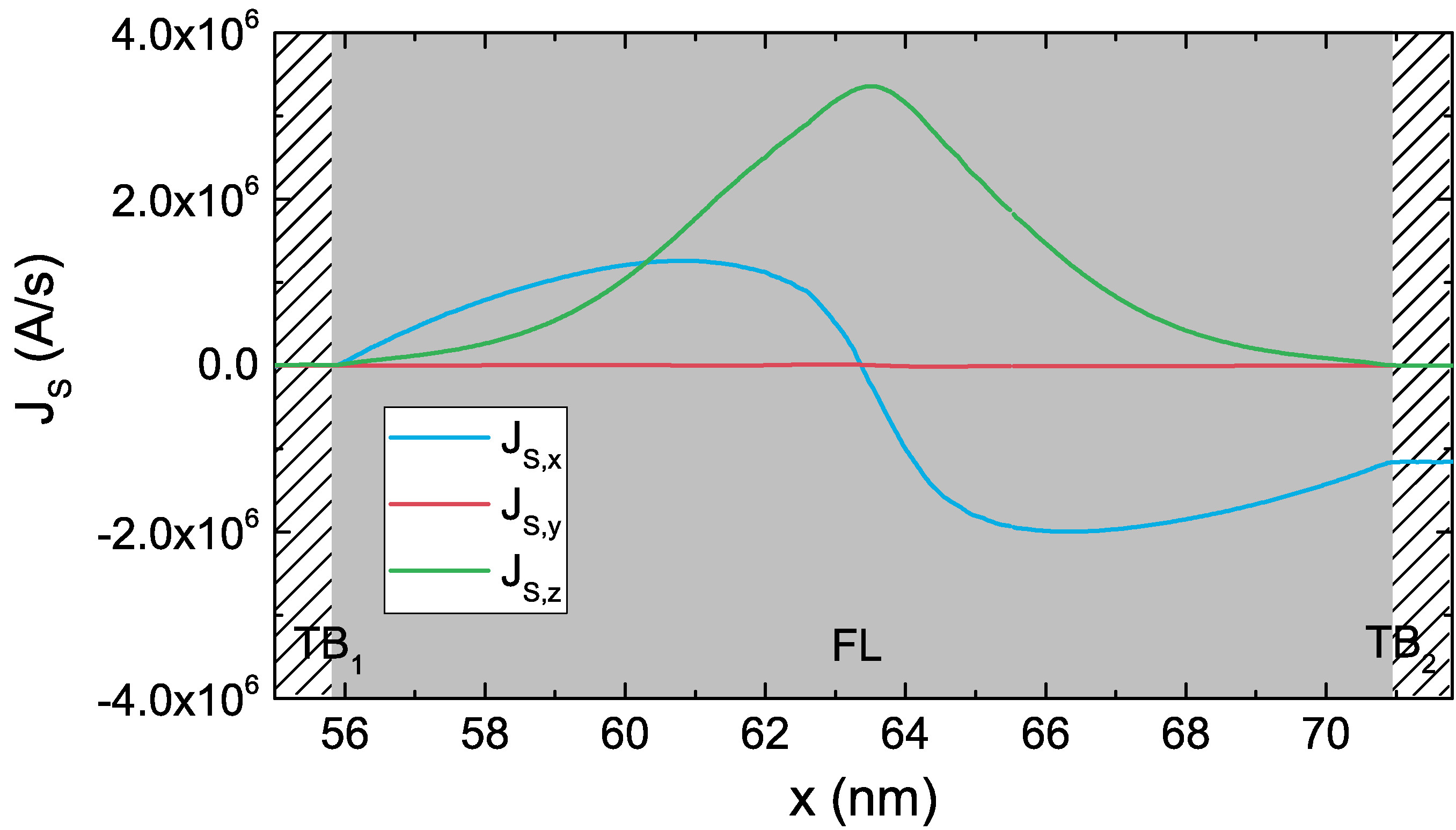
Figure 8.11: Spin currents ((a) and (c)) and torques ((b) and (d)) generated for the magnetization going from the +x- to the -x-direction over a domain wall, in the FL of the structure employed for Fig. 8.9(a). The drift-diffusion torque is compared to the one obtained from the ZL expression. The results in (a) and (b) were computed with , the
ones in (c) and (d) with .
(a)
(b)
(c)
(d)
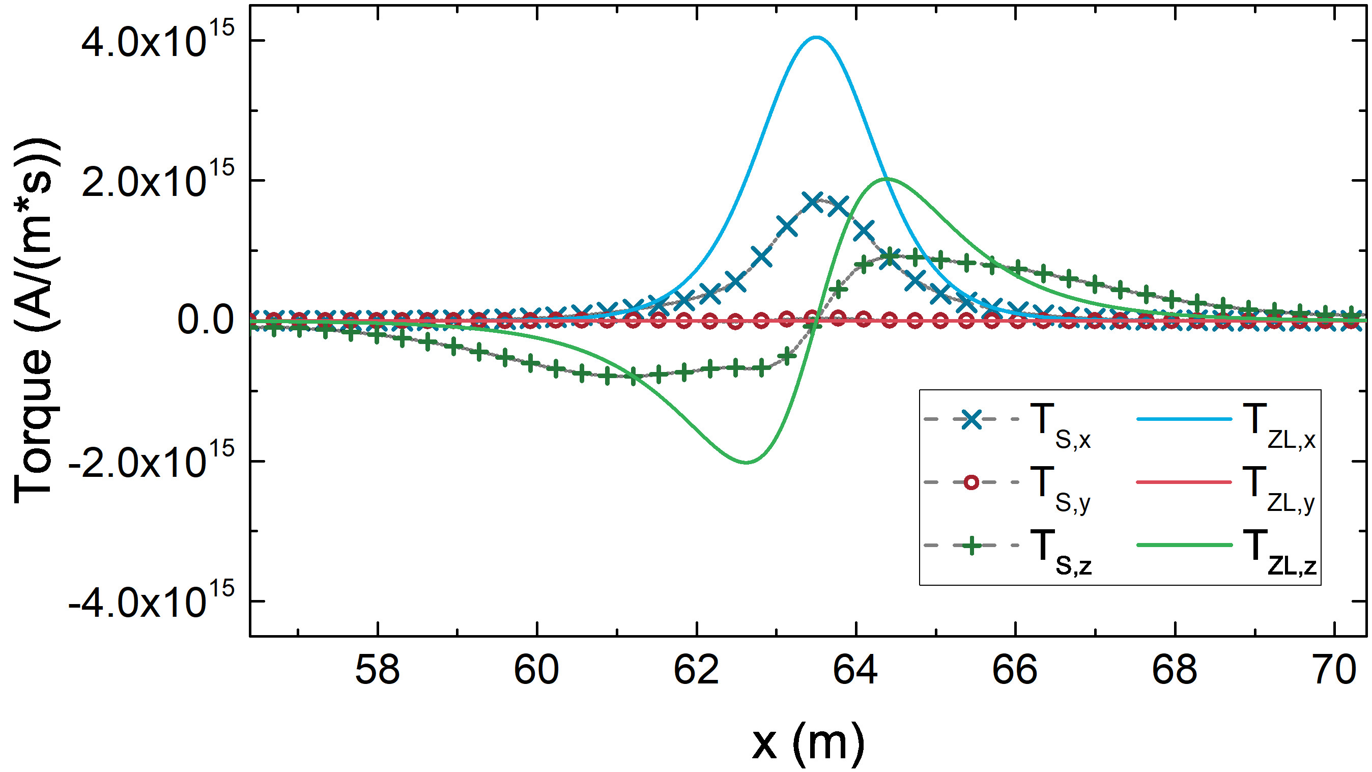
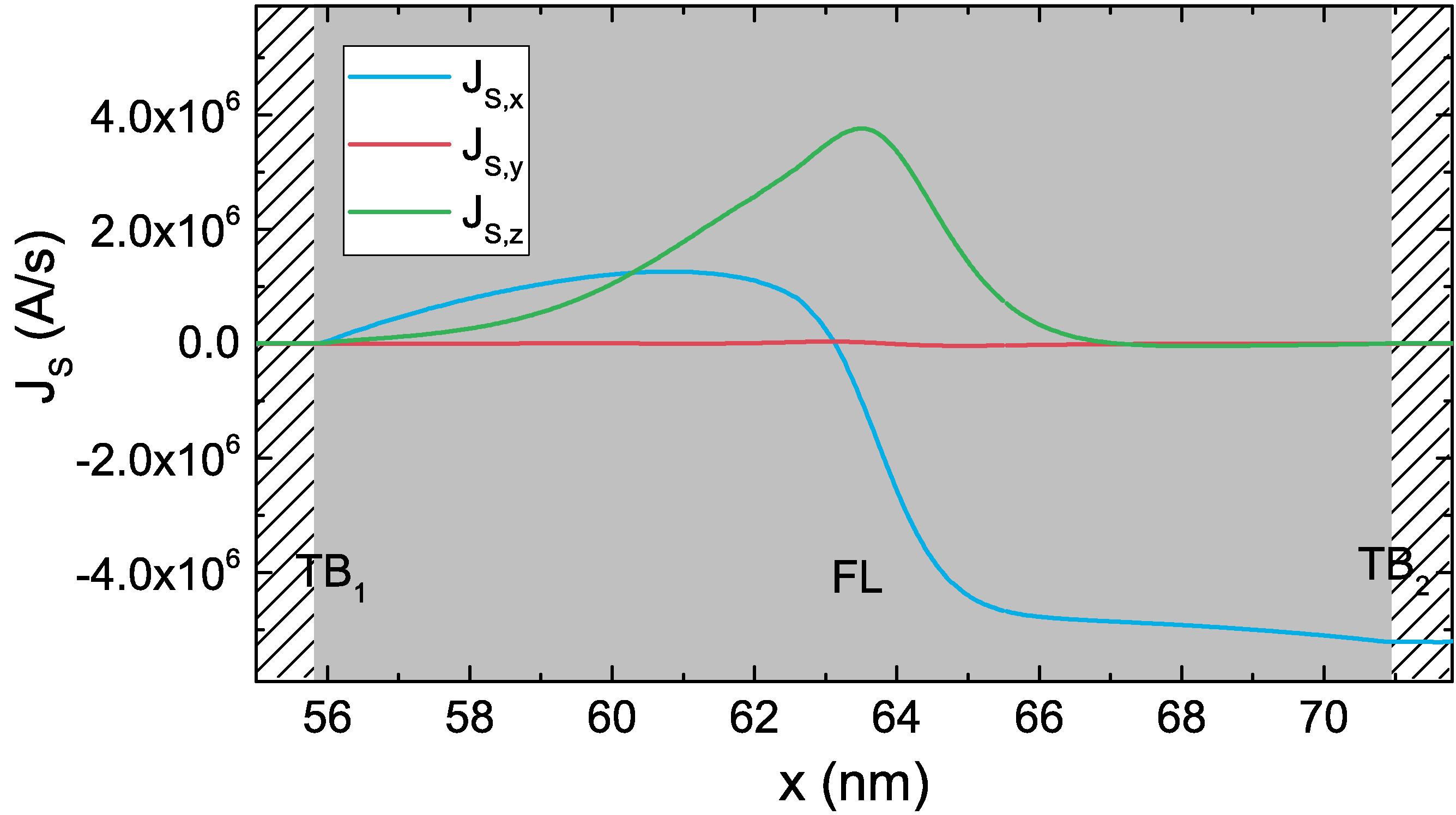
Figure 8.12: Spin currents ((a) and (c)) and torques ((b) and (d)) generated for the magnetization going from the -x- to the +x-direction over a domain wall, in the FL of the structure employed for Fig. 8.9(a). The drift-diffusion torque is compared to the one obtained from the ZL expression. The results in (a) and (b) were computed with , the
ones in (c) and (d) with .
The effect of the TBs is to modify the spin current flowing in the FM layer. The drift-diffusion solution is computed in the FL of the structure of Fig. 8.9(a), with the
complete domain wall from +x to -x in the magnetization, and . The spin current obtained in this case is reported in Fig. 8.11(a). At the
interfaces of , the RL and FL magnetization vectors are parallel, so that (8.2b) gives the tunneling spin current value in the x-direction of
. As , this
value is greater than the purely bulk one. On the opposite side, at the interface of , as only the FL interface contributes to (8.2b), the
tunneling spin current assumes the value of , which is lower than the bulk one. The difference between the tunneling and bulk spin currents is
reflected in the torques. On the left side of the domain wall, where the spin current is enhanced by the presence of , the drift-diffusion torque is slightly stronger than the ZL one, especially in the z-component. On the right
side of it, the spin current is lowered by the presence of , and the drift-diffusion torque is consequently weakened when compared to the ZL expression, valid in the bulk. In Fig. 8.11(c) and Fig. 8.11(d) the spin current and torque for are reported, respectively. In
this case, the tunneling spin current at both TBs is greater than the bulk one, so that the torque is enhanced over the whole domain wall.
The same simulations are repeated for a scenario where the magnetization in the FL is inverted, so that it goes from -x to +x over the domain wall. The sign of the current density is also inverted. The RL and FL magnetization
vectors at TB are now anti-parallel, so that the tunneling spin current goes to 0. When , the spin current at both TBs is lower than the bulk expectation, and the drift-diffusion torque is weaker
than the ZL one over the whole layer (see Fig. 8.12(a) and Fig. 8.12(b), respectively). When , the spin current tunneling across TB is instead grater than the bulk one, so that is slightly grater than on the right side of the domain wall, while still being
weaker on the left side.
The extended drift-diffusion approach clearly demonstrates that, in an MTJ with elongated ferromagnetic layers, the contributions to the torque from the tunneling process and from magnetization gradients in the structure are not
independent: the presence of the TBs influences the spin currents generated by the magnetization texture, modifying the ZL torque contribution. A unified treatment of the MTJ polarization process and FL magnetization texture is
thus required to accurately describe the torque and switching in ultra-scaled MRAM.
8.4 Switching Simulations of Ultra-Scaled MRAM Devices
The proposed approach is applied to evaluate the switching of structures reproducing recently demonstrated Ultra-Scaled MRAM devices [22]. The diameter of all the simulated
structures is 2.3 nm, and they all possess NM contacts of 50 nm. As the main interest lies in the switching behavior of the FL, the RL is kept numerically fixed, with the magnetization pointing in the positive
x-direction. The magnetization of the FL is tilted away from the perfect P or AP orientation, to emulate the destabilizing effect of a non-zero temperature on the system. The precise value employed for the tilting
angle only affects the duration of the incubation period before the start of the switching process, and does not change the overall behavior of the magnetization reversal. The resistance and polarization parameters, employed for all
the structures, are the ones reported in Table 8.3. Voltage dependence of the polarization parameters is not considered for these results.
(a)
(b)
(c)
(d)
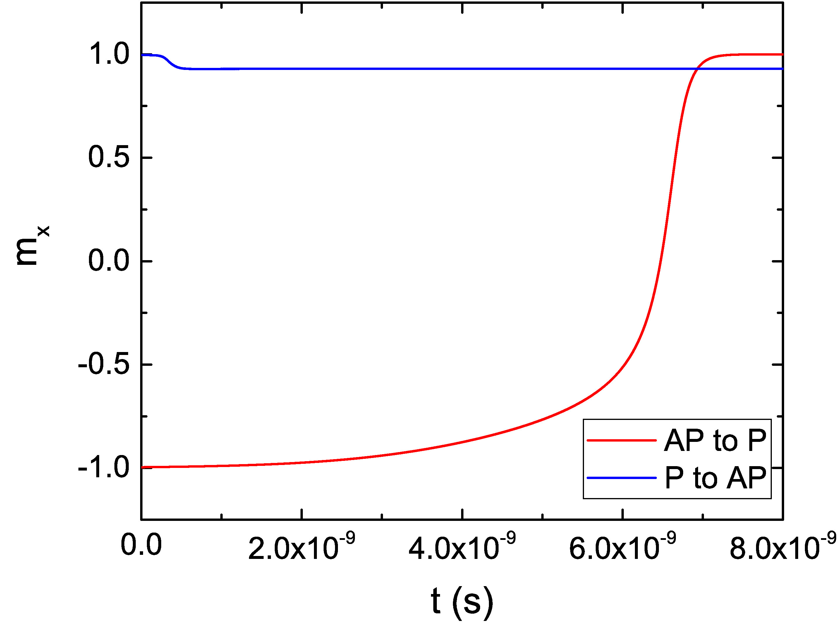
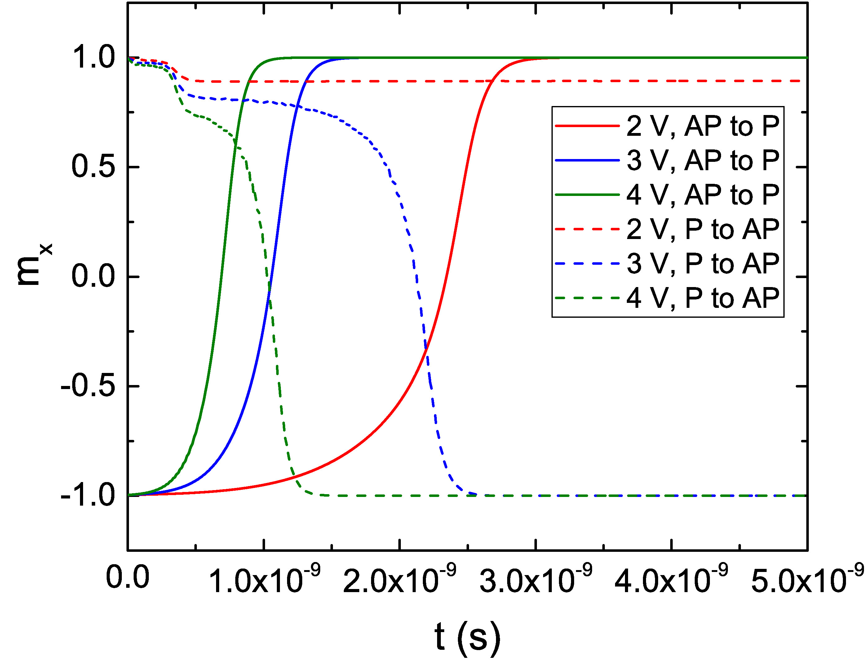
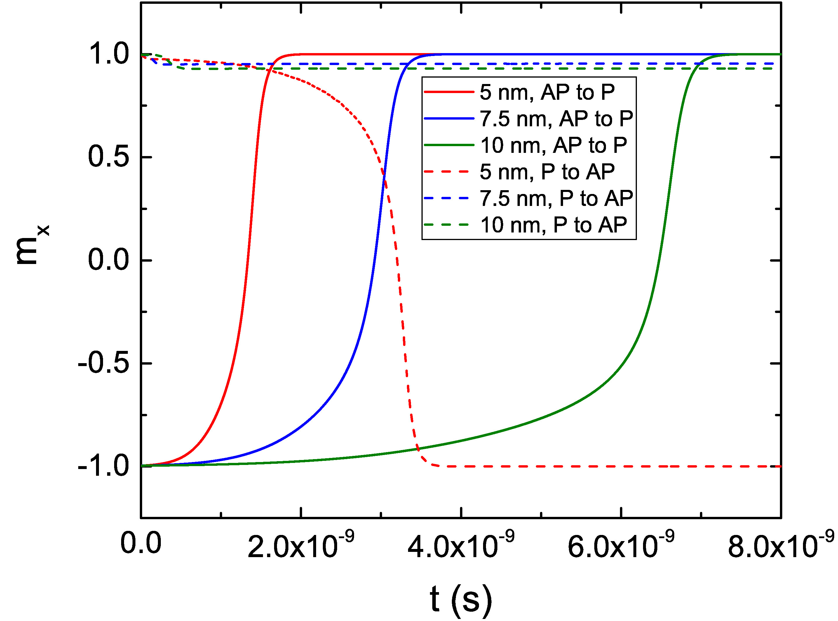
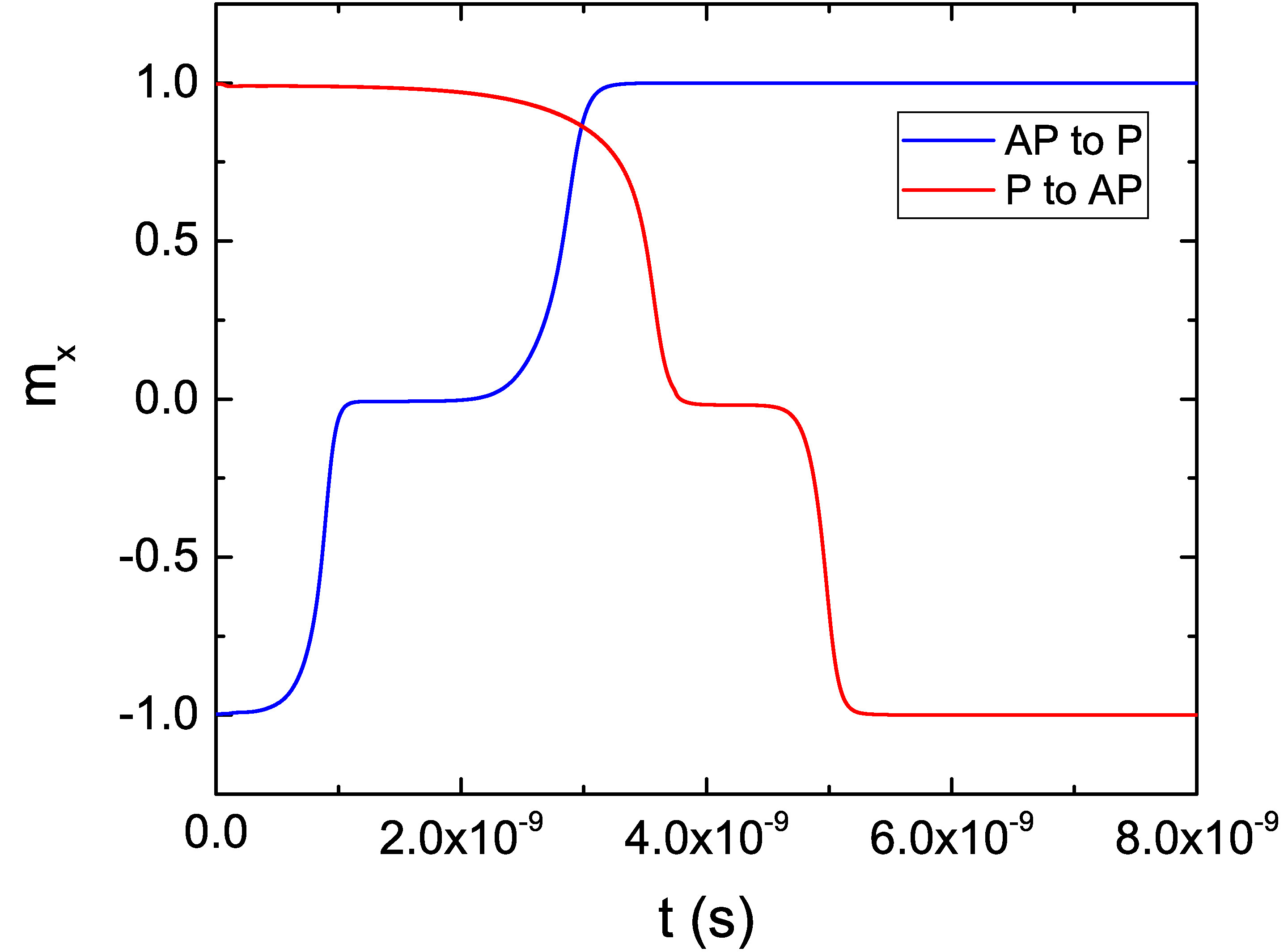
Figure 8.13: (a) Switching results for a structure with an elongated FL, for both the AP to P and P to AP scenarios, under a bias voltage of V. (b) Switching results for a structure with an elongated FL under increasing
bias voltage values. (c) Switching results for a structure with an elongated FL for several lengths of the FL. (d) Switching results for a structure with composite FL under a bias voltage of V. The figures were published
in [13].
First, switching realizations are carried out in a cell similar to the one employed for the results in the previous section, with an FL of 10 nm. The magnetization trajectories are reported in Fig. 8.13(a). A bias voltage of V is applied on the left contact for P to AP or AP to P switching, respectively. The value of the bias voltage, while being sufficient to achieve
switching for the AP to P scenario, is not enough to reverse the magnetization from P to AP. The additional stability of the parallel configuration comes from the stray field contribution of the RL, which favors it. Due to the
presence of a stronger spin current component parallel to the magnetization at the TB interface in the P state, the interaction of the Slonczewski and Zhang-Li torque contributions quickly generates a texture in the
magnetization, whose average x-component slightly deviates from the starting configuration, as evidenced by the dip in the plot during the first nanoseconds of the simulation. Despite this, the overall torque is not strong enough to
overcome the perpendicular anisotropy.
Additional simulations with increased bias values of , V and V are carried out, and the resulting magnetization trajectories are reported in Fig. 8.13(b). The increased values of the bias voltage, producing a stronger torque acting on the FL magnetization, are able to achieve switching for both configurations. Moreover, the
switching behavior of structures with FL thickness of nm and nm is investigated. The results are presented in Fig. 8.13(c). A shorter layer possesses
a reduced energy barrier separating the two magnetization configurations [53], so that the speed of AP to P switching is improved, and P to AP reversal is achieved in the case of
the nm layer.
The switching performance can be improved by employing a structure where the FL is split into two parts of nm length by an additional MgO layer (TB), presented in the middle of Fig. 1.2. The addition of an MgO layer boosts the overall stability of the cell because of an increased interface anisotropy contribution, while the two parts of the FL have a preferred aligned
configuration because of the stray field they exert on one another [22]. The presented approach is employed to carry out switching simulations in such a structure, under a bias
voltage of V. TB is taken to possess the same conductance of TB, and a polarization parameter [22]. The
results are presented in Fig. 8.13(d). The plot evidences how the switching process is overall faster in the composite structure as compared to the one with a single elongated layer,
and that P to AP switching is achieved for lower values of the bias voltage. Both the AP to P and P to AP results present clear steps in the magnetization trajectories.
(a)
(b)
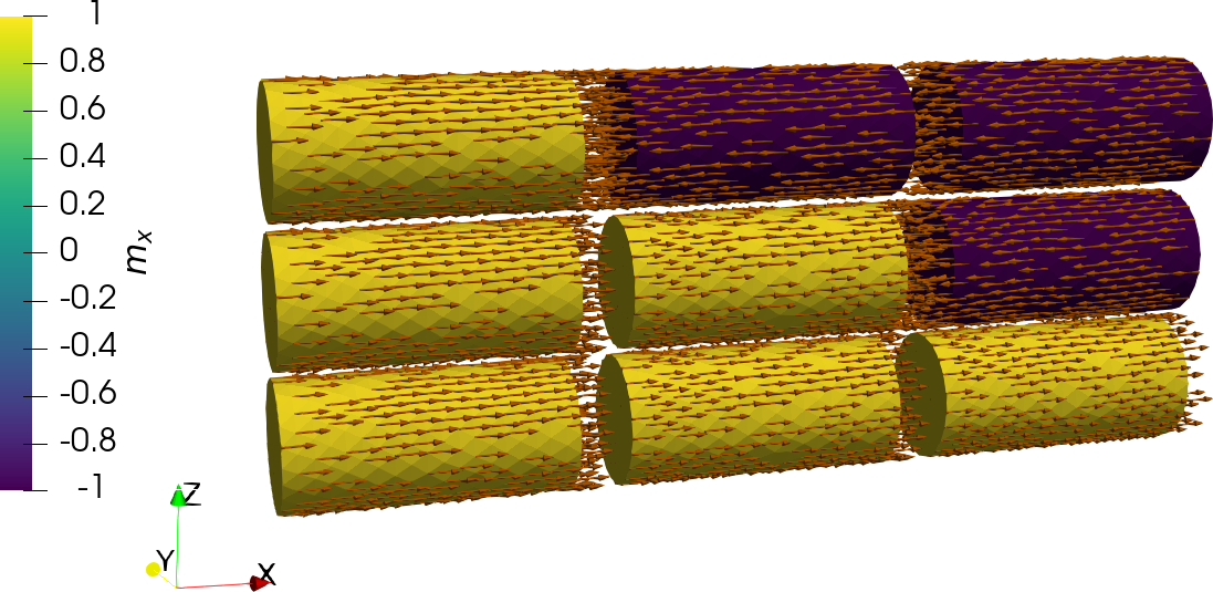
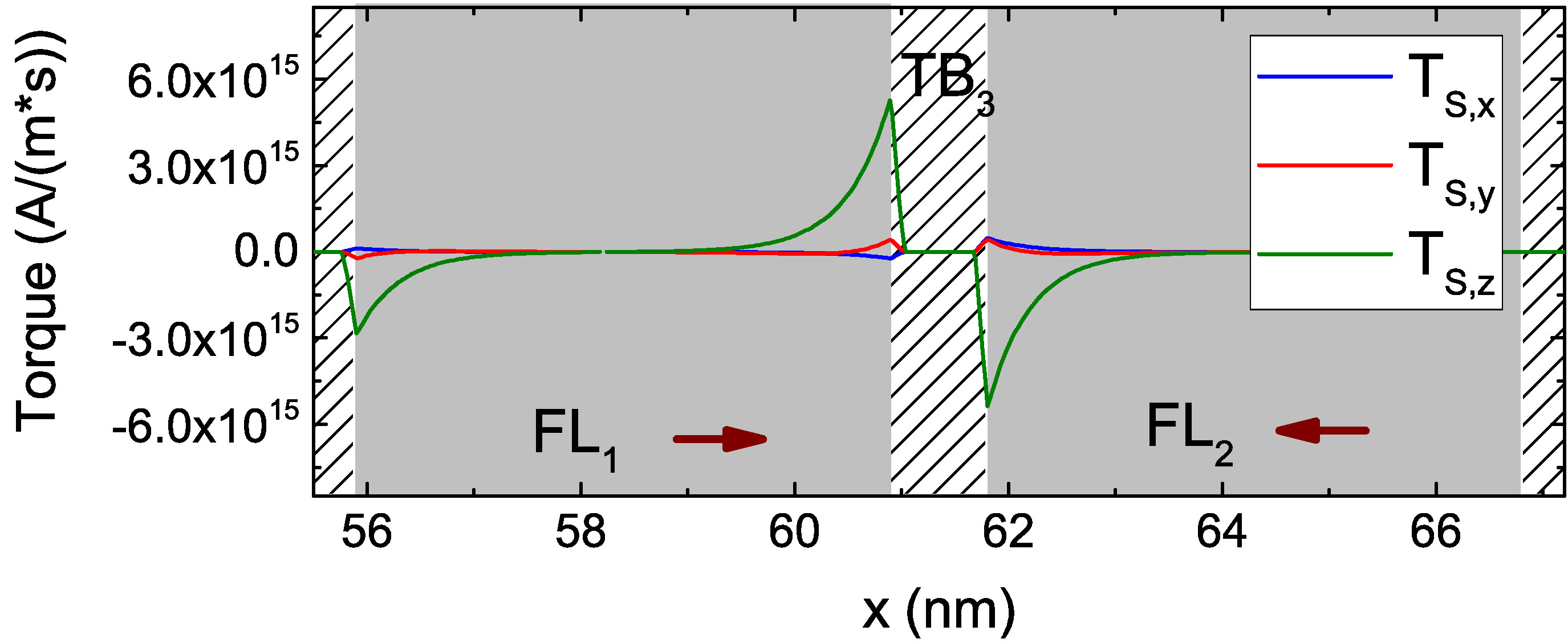
Figure 8.14: Switching stages of an ultra-scaled STT-MRAM cell with composite FL, showcasing how the different parts of the FL switch one at a time. The RL is the first section on the left of the structure, while the
second and third sections are the two parts of the FL (from left to right, FL and FL, respectively). AP to P switching is presented in (a), while P to AP switching in (b). The figures were published in [13].
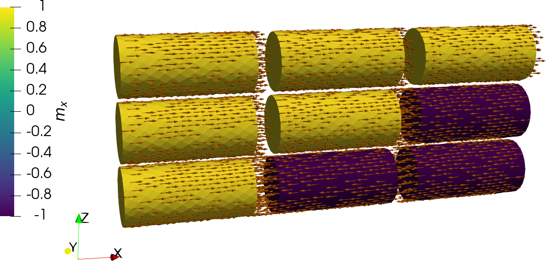
(a)
(b)
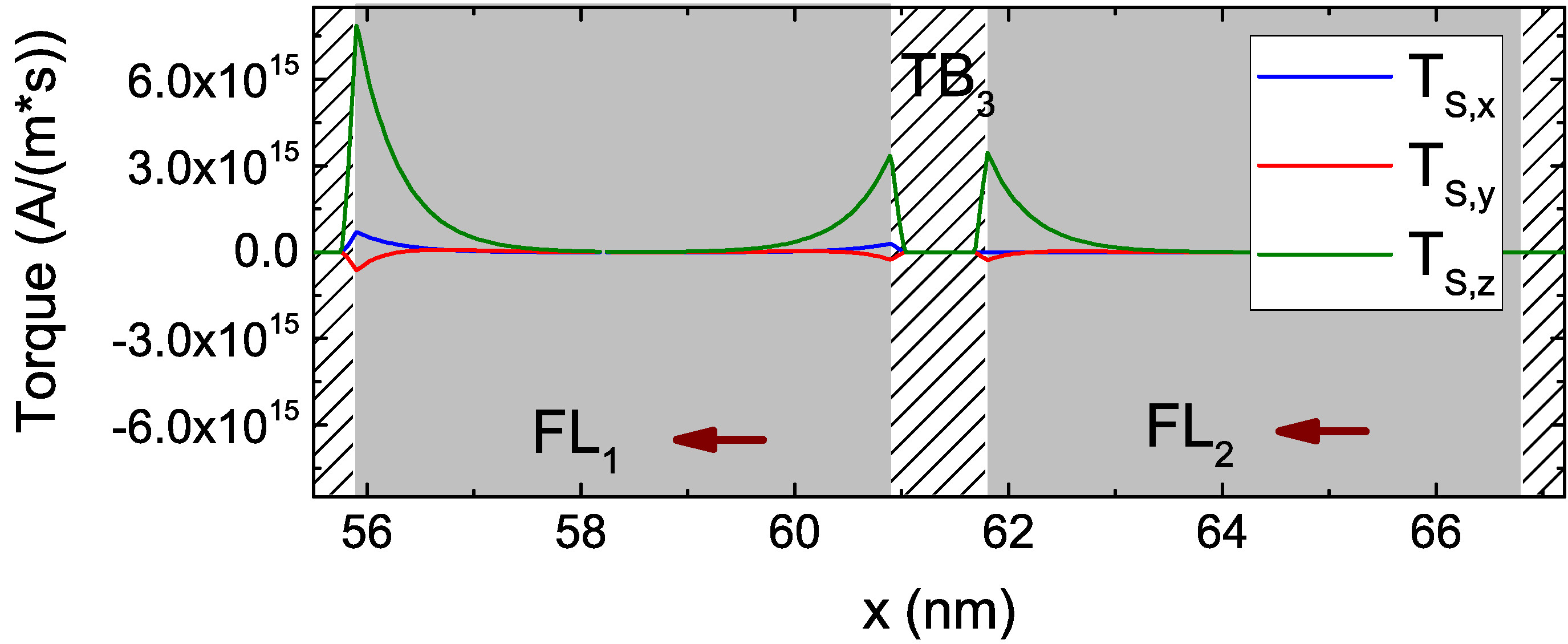
Figure 8.15: (a) Torque configuration near the beginning of the AP to P switching. The torques coming from the RL and FL act together to switch FL. The arrows represent the magnetization vector in the two FL
sections. (b) Torque configuration after the first section of the composite FL has almost reached the plateau at . The torques coming from the RL and FL keep FL stable, while FL is switched by the
torque acting on it from FL.
These steps are best explained by looking at their respective magnetization state, reported in Fig. 8.14. The improved performance of this structure comes from the composite
nature of the FL, allowing for its different sections to be switched one at a time. In the AP configuration, the RL exerts a torque on the first part of the FL (FL) to push it in the positive x-direction, parallel to it. At the
same time, the second part of the FL (FL) also exerts a torque on FL to push the magnetization to the positive x-direction, so that it is anti-parallel to FL. Both torques’ contributions act in the same direction,
causing FL to switch first and fast. At the same time, the torque acting from FL towards FL favors the two magnetization vectors to be parallel, keeping FL in its original orientation. However, after the
magnetization of FL has switched, the torque acting on FL changes its sign, forcing it to switch as well. As the torque acts only from FL, the magnitude is smaller than that acting in the first part of the
switching process, resulting in a slower reversal of the FL magnetization.
The three stages of AP to P switching are showcased in Fig. 8.14(a). When going from P to AP, the opposite process happens. The torque acting from FL on
FL is opposite to that from the RL, while the torque acting from FL on FL is favoring magnetization reversal, so that FL switches first. As only the torque from FL is acting, the switching of
FL is relatively slow. After FL has switched, the torque contributions from FL and the RL act on FL in the same direction, completing the switching fast. The three stages of P to AP reversal are shown in
Fig. 8.14(b). Fig. 8.15 provides a visual representation of the torques acting at the beginning and during the
first step of the AP to P switching. The obtained switching time and the applied bias voltage are in line with the experimentally reported results [22], and show how the
presented approach can be applied to investigate the switching behavior of emerging MRAM devices.
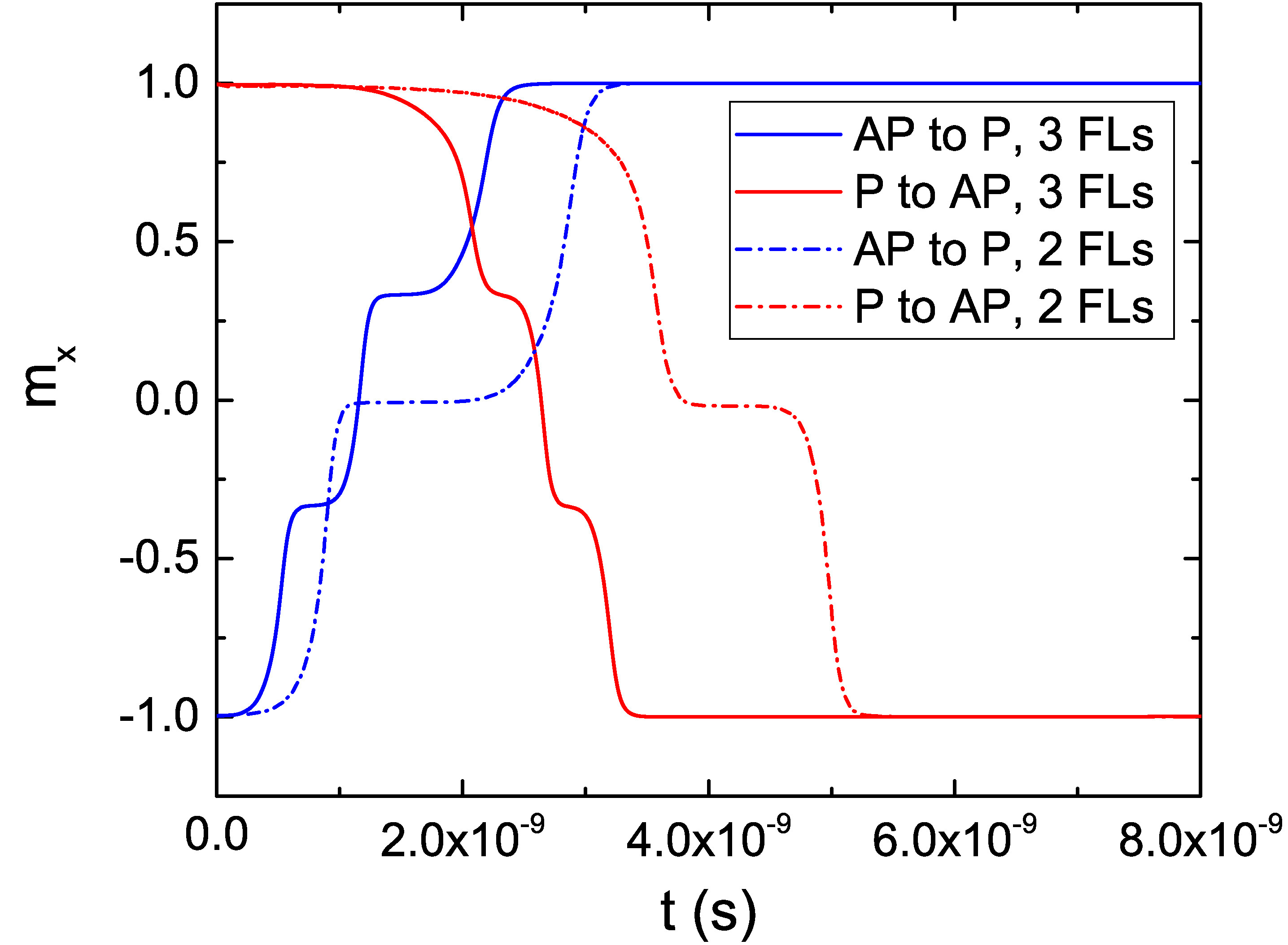
Figure 8.16: Switching results for a structure with three FL segments, for both the AP to P and P to AP scenarios, under a bias voltage of 1.5 V (solid line). The magnetization trajectories are compared to the ones obtained
in the structure with two FL segments (dash-dotted lines). The figure was published in [13].
In order to further analyze the performance of a composite FL, simulations are performed to investigate the switching behavior of an MRAM cell with three FL segments. These structure has an additional TB (TB) in the
FL, with the same properties of TB. The switching realizations are performed in a cell with segments of nm thickness, with a similar total length of the FL as the previous two. The structure is reported on the
bottom of Fig ,1.2. The results for both AP to P and P to AP switching are reported in Fig. 8.16, for a bias voltage of V. The switching process is qualitatively similar to the one of the structure with two FL segments, with the three sections of the FL switching one at a time. In the AP configuration, the torque coming from the RL
and FL causes the fast switching of FL to the positive x-direction. At this point, the torque coming from FL and the third part of the FL (FL) causes the magnetization in FL to also switch fast.
Finally, as only the torque coming from FL acts on FL, the latter has a slower magnetization reversal which completes the switching process. When going from P to AP, as is the case for the structure with two FL
segments, the opposite process happens. The torques acting on FL and FL from the adjacent layers compensate each other, and only the torque acting from FL on FL is able to cause the magnetization
reversal of the latter. At this point, the torque acting from FL and FL on FL becomes additive, so that FL switches faster. This is finally followed by the fast switching of FL, as the torque
contributions coming from the RL and FL push its magnetization towards the negative x-direction. Fig. 8.16 also shows that the complete switching process is faster in the structure
with three FL segments, for both AP to P and P to AP realizations. This is in line with the easier switching of shorter layers observed in Fig. 8.13(c). The simulations show
that the increased number of segments provides an advantage in terms of switching time and bias, and the multiple magnetization states reached during the switching process make these structures promising candidates as multi-bit
memory cells.
8.5 Ballistic Spin Current Terms
(a)
(b)
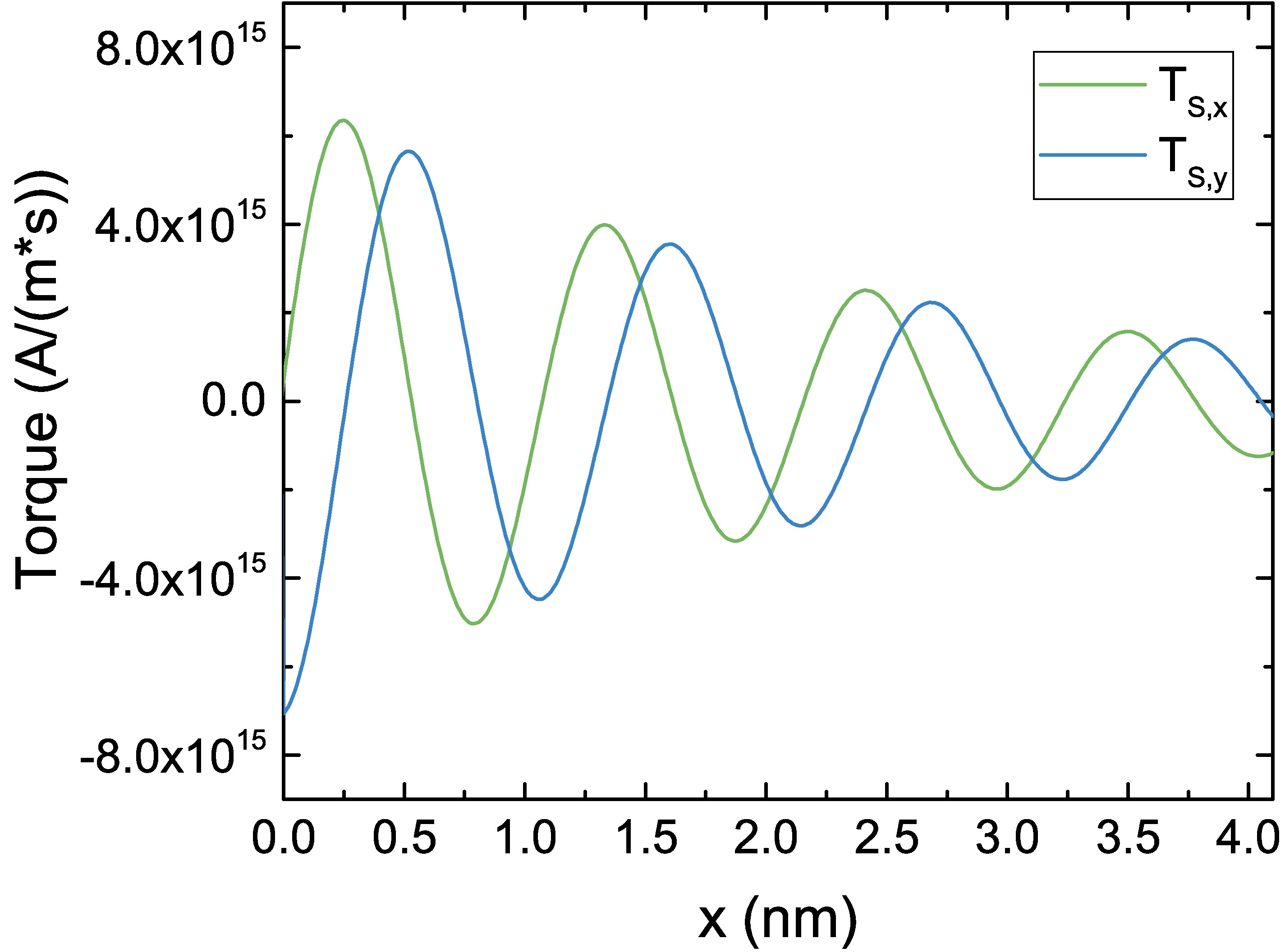
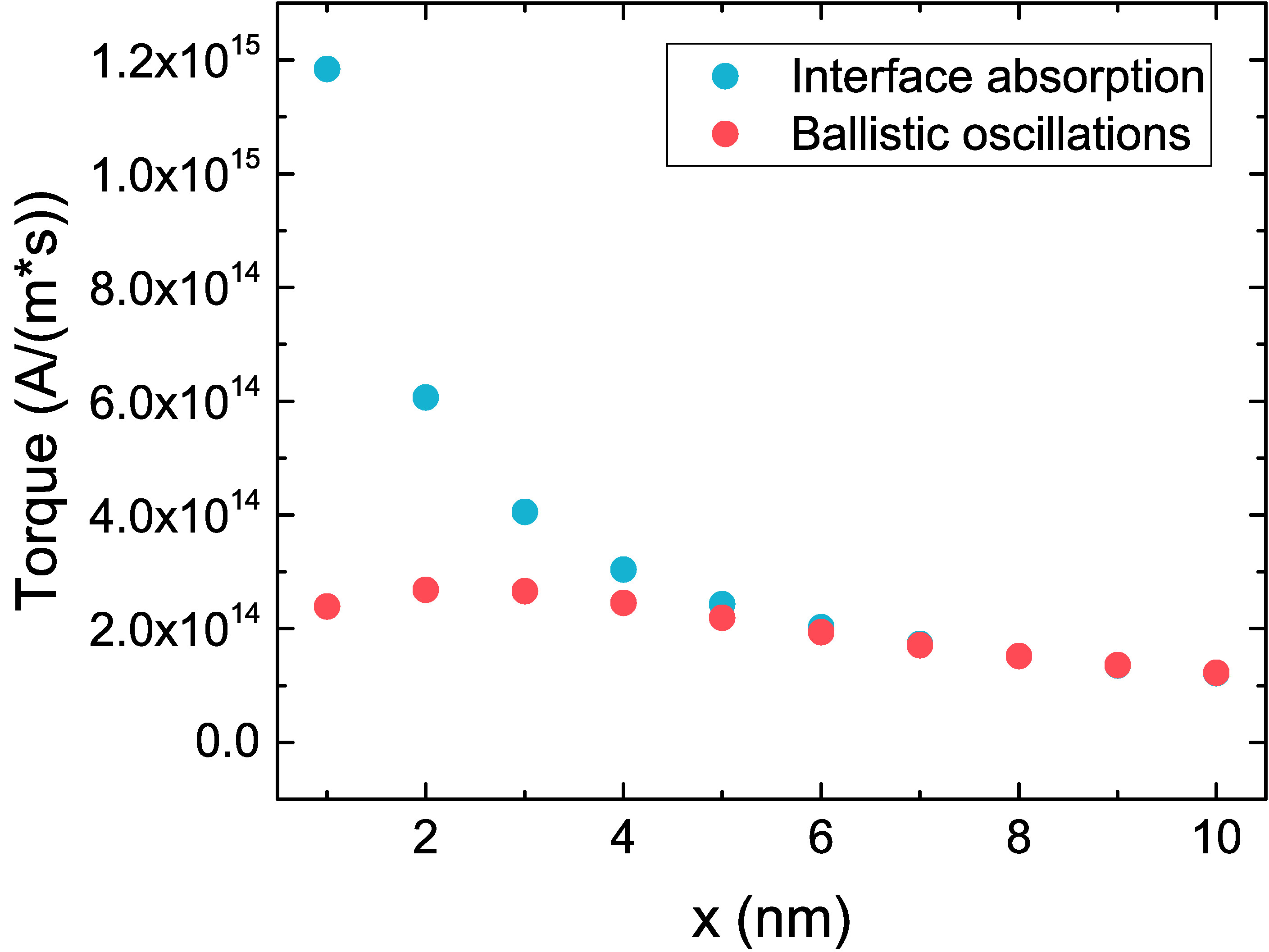
Figure 8.17: (a) Torque computed with the inclusion of ballisitic corrections to the spin current in a semi-infinite FL. Results are in qualitative agreement with [99]. (b)
Comparison of the thickness dependence of the total damping-like torque acting on the FL in the presence of fast interface absorption or ballistic and oscillating behavior of the transverse spin accumulation components. The figures
were published in [164].
Recent analytical investigations of the behavior of the torque in the ballistic regime based on the NEGF formalism predict a complex absorption pattern for the transverse components, with an oscillatory dependence of the spin
torque on the distance from the TB interface [99]. As these complex oscillatory behavior is ballistic in origin, it can only be reproduced by considering the additional spin
current terms presented in equation (6.36b). In this case, the spin current expression to be employed in equation (6.38a) becomes
where is a magnetization dependent tensor, with the components
The system of equations presented in Section A.2 of the Appendix can be adapted to the presence of the additional terms, as detailed in Section A.3. In Fig. 8.17(a) the resulting torque computed using nm, nm, and the
electron relaxation length nm in a semi-infinite FL is shown. The RL magnetization points in the x-direction, the one of the FL points in the z-direction. A current density of A/m is flowing in the x-direction. With these choice of absorption lengths, the oscillating behavior of the torque components is in qualitative agreement with the results reported in [99].
The presence of such a pattern has an effect on the total torque exerted on the FL, obtained from (7.4). In Fig. 8.17(b), a comparison of the dependence of the total damping-like torque computed with the fast absorption of the transverse components, previously presented, and with the oscillating torque
of Fig. 8.17(a) is depicted. For long FLs, both approaches show an inverse dependence of the torque on the thickness of the FL. Below 4 nm, however, the transverse
components are not completely absorbed in the ballistic approach, so that the dependence of the torque on the FL thickness becomes more complex, and its value is reduced. The observed difference between the total torque acting
in short FLs can provide a valid benchmark to establish which of the two approaches is most suitable to accurately describe the switching behavior of STT-MRAM devices.